Notes on Machine Learning 14: Markov Models

(ML 14.1) Markov models - motivating examples

“The future is independent from the past, given the present.”

Everything that you would want to know to predict the futute is alraedy encoded in the current state of the world.

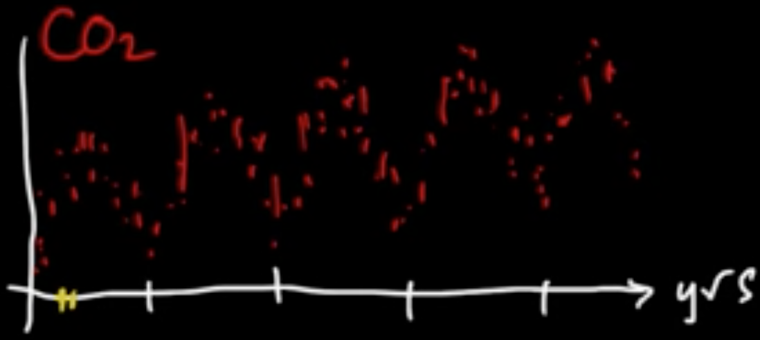
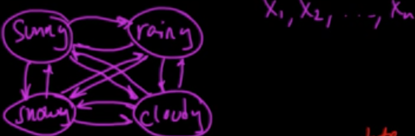
• Temporal data (sequence of data): e.g. weather, finance, language, music, etc.

• Applications: speech recognition, music composition, (Mark V. Shaney)

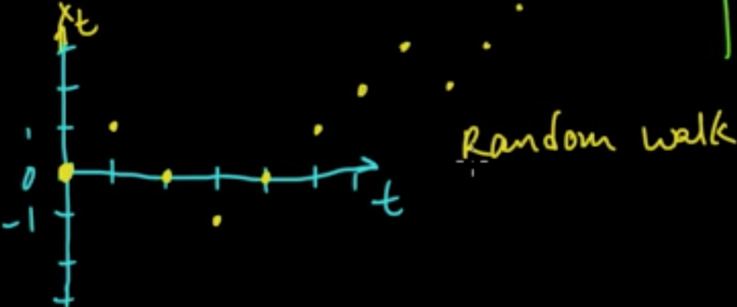
(Sequential) Data: $D = (x_1, \ldots, x_n)$.
Model data as random variables: $X_1, \ldots, X_n$

• iid? No
• Everything depends on everything else. $\leadsto$ intractable problem
• $X_t$ depends on $X_{t-1}, X_{t-2}, \ldots, X_{t-m}$ for fixed $m$

The simplest case $m=1$ (for the last line) leads to the notion of Markov chain

(ML 14.2) (ML 14.3) Markov chains (discrete-time)

Simplifying assumptions: Discrete time and discrete space.

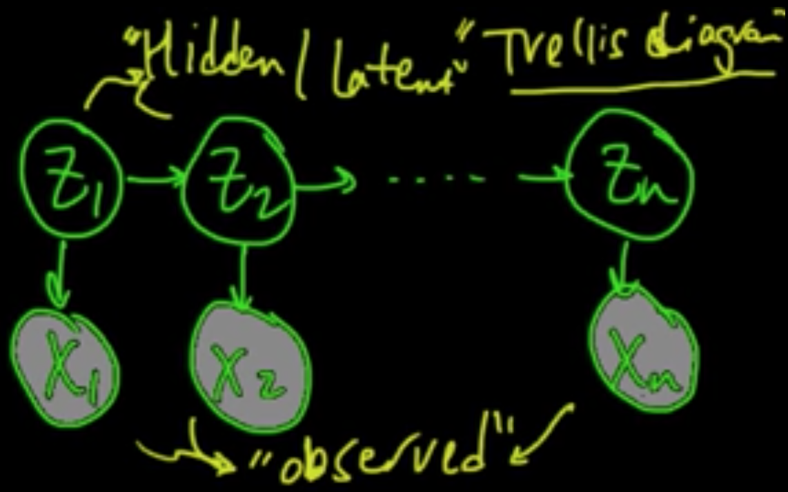
Definition. Discrete ranndom variables $X_1, \ldots, X_n$ form a (discrete-time) Markov chain if they respecs the following graphical model

i.e., $p(x_t \vert x_1, \ldots, x_{t-1}) = p(x_t \vert x_{t-1})$.

Implication:

2nd order Markov chain.

Continuous-time Markov chain.

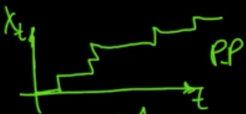
Continuous-space Markov chain.
e.g. 1st order autoregressive model

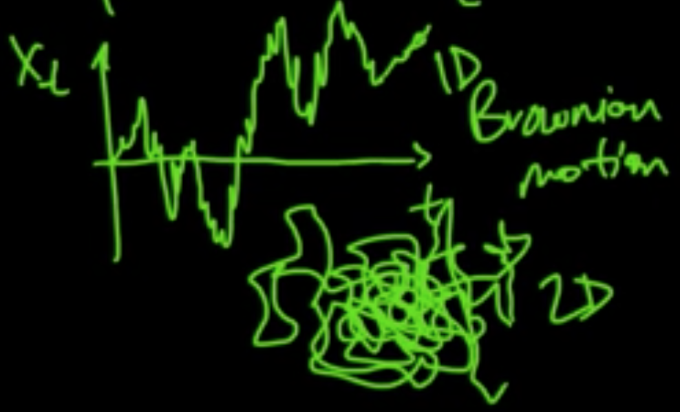
Continuous-time and continuous-space Markov model.
e.g. Brownian motion

Example 1 (discret-time and discrete-space Markov chain).

Example 2 (discret-time and discrete-space Markov chain).

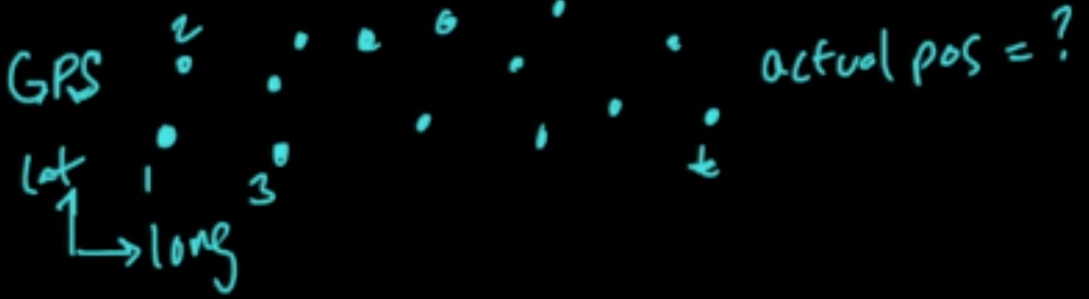
BUT, can’t expect to perfectly observe complete true state of the system!
Answe: There is hidden info. Model with hidden/latent variables. $\leadsto$ HMM

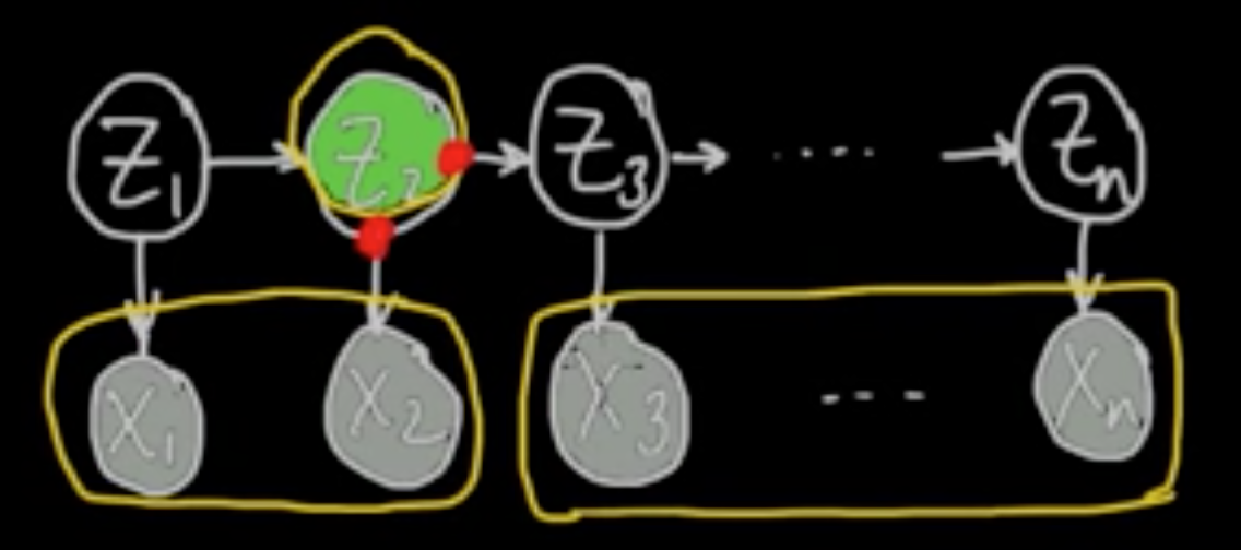
(ML 14.4) (ML 14.5) Hidden Markov models

Model.
$Z_1, \ldots, \in \{1, \ldots, m\}$
$X_1, \ldots, X_n \in \mathscr{X}$ (e.g. discrete, $\mathbb{R}, \mathbb{R}^d$)
$D = (x_1, \ldots, x_n)$

$p(x_1, \ldots, x_n, z_1, \ldots, z_m) = p(z_1)p(x_1\vert z_1)\prod_{k=2}^np(z_k\vert z_{k-1})p(x_k\vert z_k)$

An application of HMM could be hand writing recognition.

Parameters.

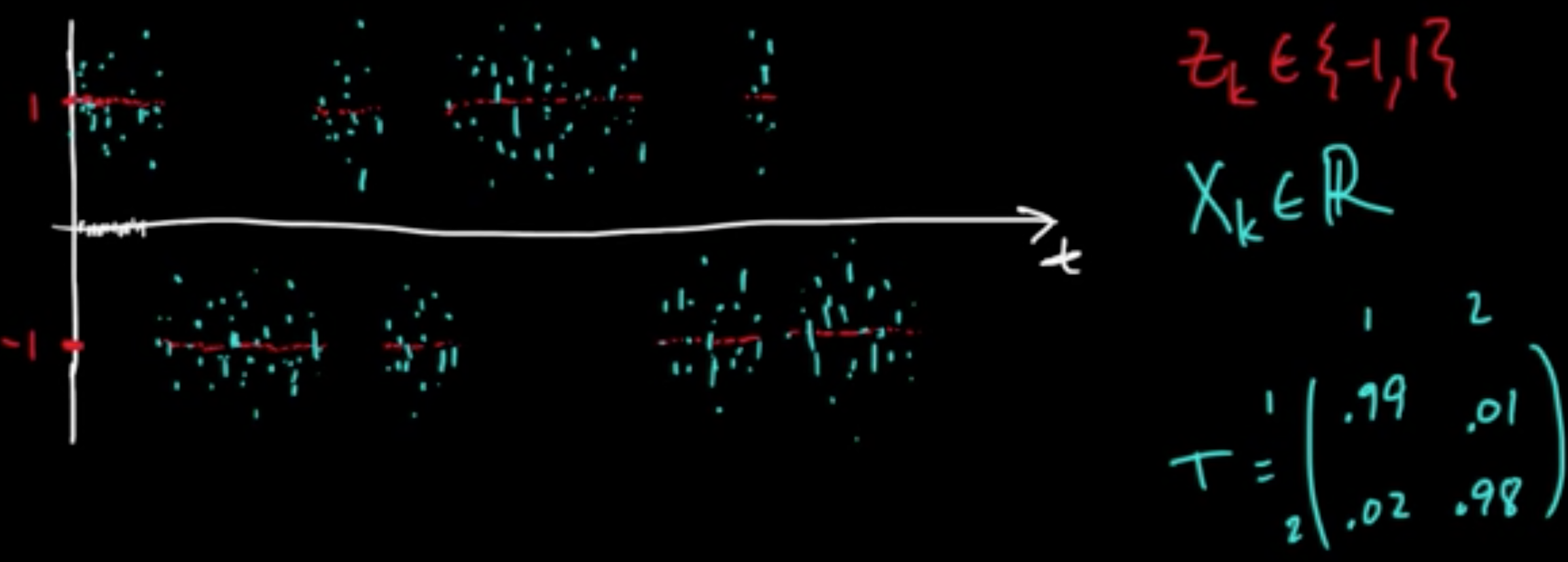
• Transition probabilities: $T(i, j) = P(Z_{k+1} = j \vert Z_k = i)$ ($i,j \in \{1, \ldots, m\}$)
• Emission probabilities: $E_i(x) = p(x \vert Z_k=i)$ for $i \in \{1,\ldots, m\}$, $x \in \mathscr{X}$ (pdf)
  or $E_i(x) = P(X_k = x \vert Z_k=i)$ (pmf)
• Initial distribution: $\pi(i)=P(Z_1= i)$, $i \in \{1, \ldots, m\}$

$p(x_,\ldots, x_n, z_1, \ldots, z_M) = \pi(z_1)E_{Z_1}(x_1)\prod_{k=2}^n T(z_{k-1}, z_k)E_{Z_k}(x_k)$

Remark. $E_i$’s pretty arbitrary.

Example.

(ML 14.6) Forward-Backward algorithm for HMMs

“Dynamic Programming” introduced by Richard Bellman

Assume $p(x_k \vert z_k), p(z_k\vert z_{k-1}), p(z_1)$ known.

Let $x = (x_1, \ldots, x_n)$, $x_{i:j} = (x_i, x_{i+1}, \ldots, x_j)$, $x=x_{1:n}$, $x_{k+1:n}=(x_{k+1},\ldots, x_n)$

F/B: Compute $p(z_k \vert x)$

Forward algorithm: Compute $p(z_k, x_{1:k})$ $\forall k \in \{1, \ldots, n\}$

Backward algorithm: Compute $p(x_{k+1:n}\vert z_k)$ $\forall k \in \{1, \ldots, n\}$

$p(z_k\vert x) \propto_{z_k} p(z_k, x) = p(x_{k+1:n \vert z_k, x_{1:k}})p(z_k,x_{1:k})$

What you can do:

• Inference: $P(Z_k \neq Z_{k+1} \vert x)$ “change detection”
• Estimate parameters (“Baum-Welch”)
• Sampling from posterior distribution $z \vert x$

(ML 15.1) Newton’s method (for optimization) - intuition

2nd order method!

(Gradient descent $x_{t+1} = x_t - \alpha_t \nabla f(x_t)$ : 1st order method)

Analogy (1D).

• zero-finding: $x_{t+1} = x_t - \frac{f(x_t)}{f’(x_t)}$

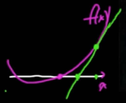
• min./maximizing: $x_{t+1} = x_t - \frac{f’(x_t)}{f’‘(x_t)}$

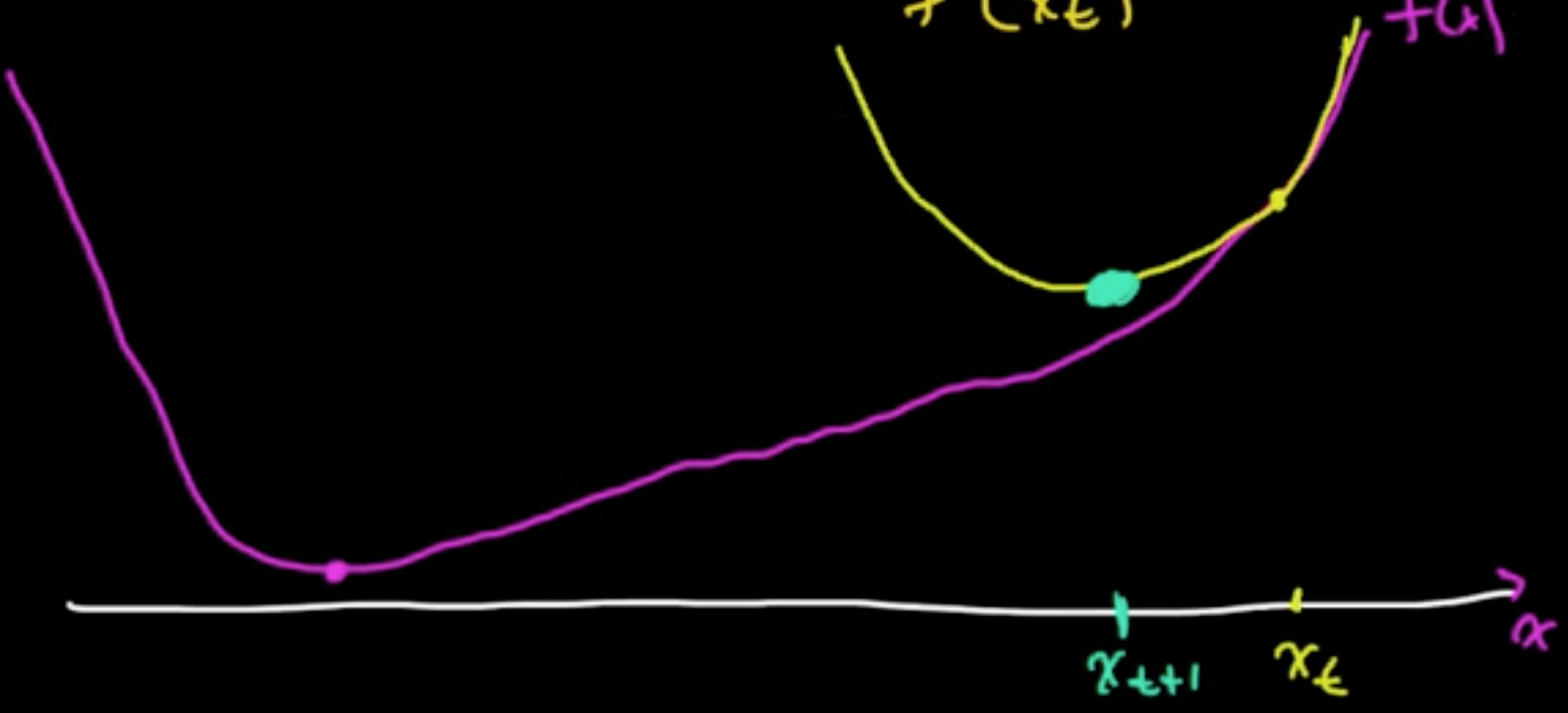
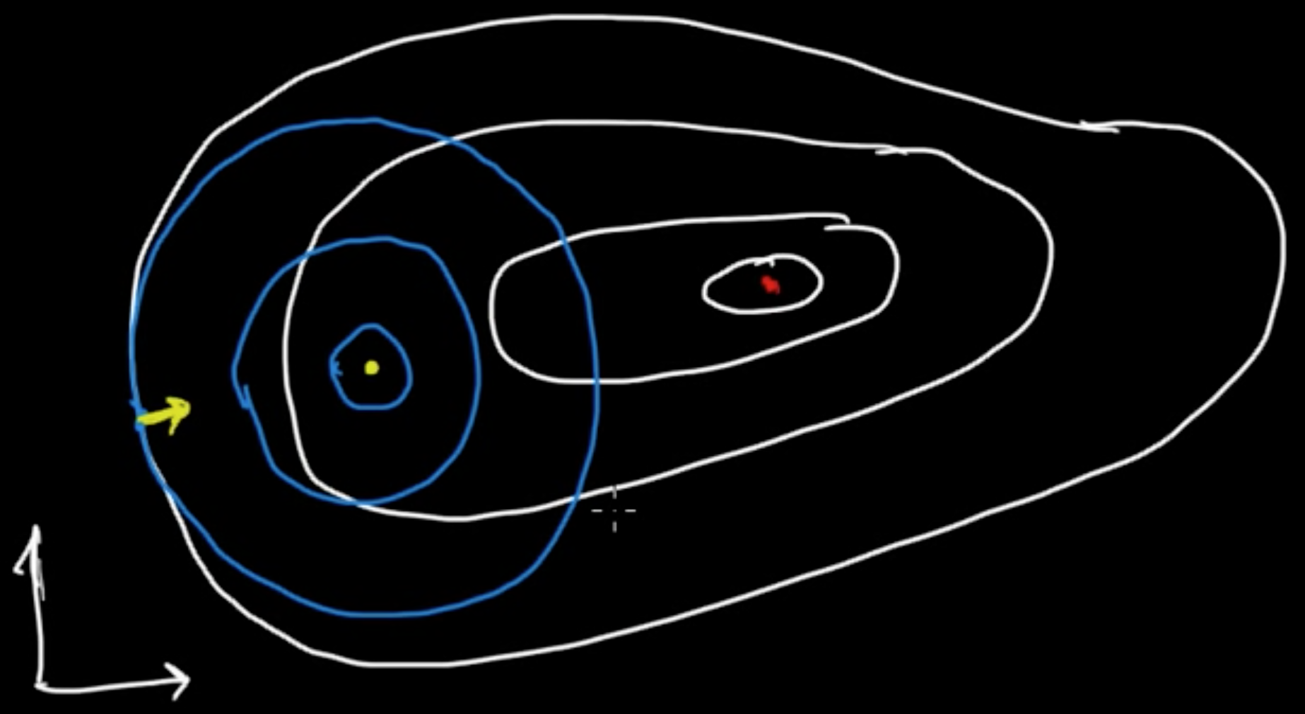
(ML 15.2) Newton’s method (for optimization) in multiple dimensions

Idea: “Make a 2nd order approximation and minimize tha.”

Let $f: \mathbb{R}^n \rightarrow \mathbb{R}$ be (sufficiently) smooth.

Taylor’s theorem: for $x$ near a, letting $g = \nabla f(a)$ and $H = \nabla^2f(a) = \left(\frac{\partial^2}{\partial x_i \partial x_j}f(a)\right)_{ij}$,

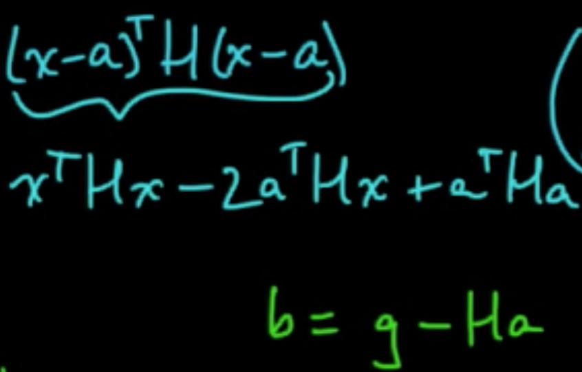
Minimize: $0 = \nabla q = Hx + b \Rightarrow x = -H^{-1}b = a -H^{-1}g$

Critical to check: $\nabla^2 q = H$ $\Rightarrow$ minimum if $H$ is PSD.

Algorithm.

• Initialize $x \in \mathbb{R}^n$
• Iterate: $x_{t+1} = x_t - H^{-1}g$ where $g = \nabla f(x_t), H = \nabla^2 f(x_t)$

Issues.

1. $H$ may fail to be PSD. (Option: switch gradient descent. A smart way to do it: Levenberg–Marquardt algorithm)
2. Rather than invert $H$, sove $Hy = g$ for $y$, then use $x_{t+1} = x_t - y$. (More robust approach)
3. $x_{t+1} = x_t - \alpha_t y$. (small “step size” $\alpha_t>0$)

(ML 16.6) Gaussian mixture model (Mixture of Gaussians)

$Z \in \{e_1, \ldots, e_m\}$, standard vectors in $\mathbb{R}^m$ ($Z$ is “latent” variable)
$P(Z = e)k = \alpha_k$
Given $Z = e_k$,
$X \sim N(\mu_k, C_k)$
where $\mu_1, \ldots, \mu_m \in \mathbb{R}^d$ and $C_1, \ldots, C_m$ $d\times d$ cov. matrices.

Marginal distribution:
$\begin{aligned} p(x) & = \sum_z p(x\vert z)p(z) \\ & = \sum_{k=1}^m P(Z = e_k) P(x \vert Z = e_k) \\ & = \sum_{k=1}^m \alpha_k N(x \vert \mu_k, C_k) \end{aligned}$

The $\alpha_k$ are called the mixing coefficients.

Joint distribution:

where $z = (z_1, \ldots, z_m)$

On the other hand,

Note that $P(Z = e_k \vert x) = \mathbb{E}(I(Z=e_k)\vert X=x)$.

(ML 17.1) Sampling methods - why sampling, pros and cons

Why is sampling so powerful and useful?

• For approximating expectations ($\leadsto$ estimate statistics / posterior infernce i.e. computing probability)
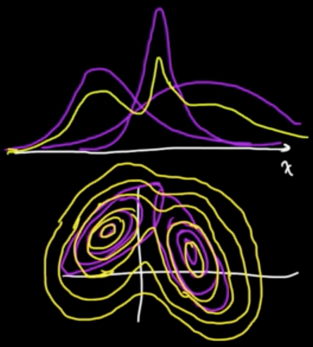
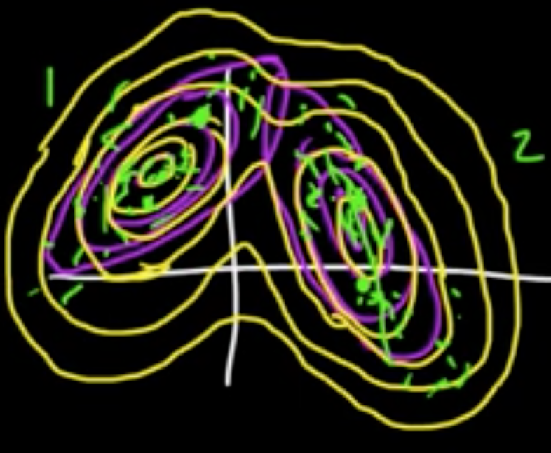
• For visualization of typical draws from a distribution of interest

Why expectations?

• Any probability is an expectation: $P(X \in A) = E(I_{X \in A})$.
• Approximation is needed for intractable sums/integrals (can be expressed as expectations)

Pros.

• Easy (both to implement and to understand)
• General purpose (widely applicable)

Cons.

• Too easy (used inappropriately)
• Slow (usually need lots of samples)
• Getting “good” samples may be dificult
• Difficult to assess the performance of methods (e.g. MCMC)

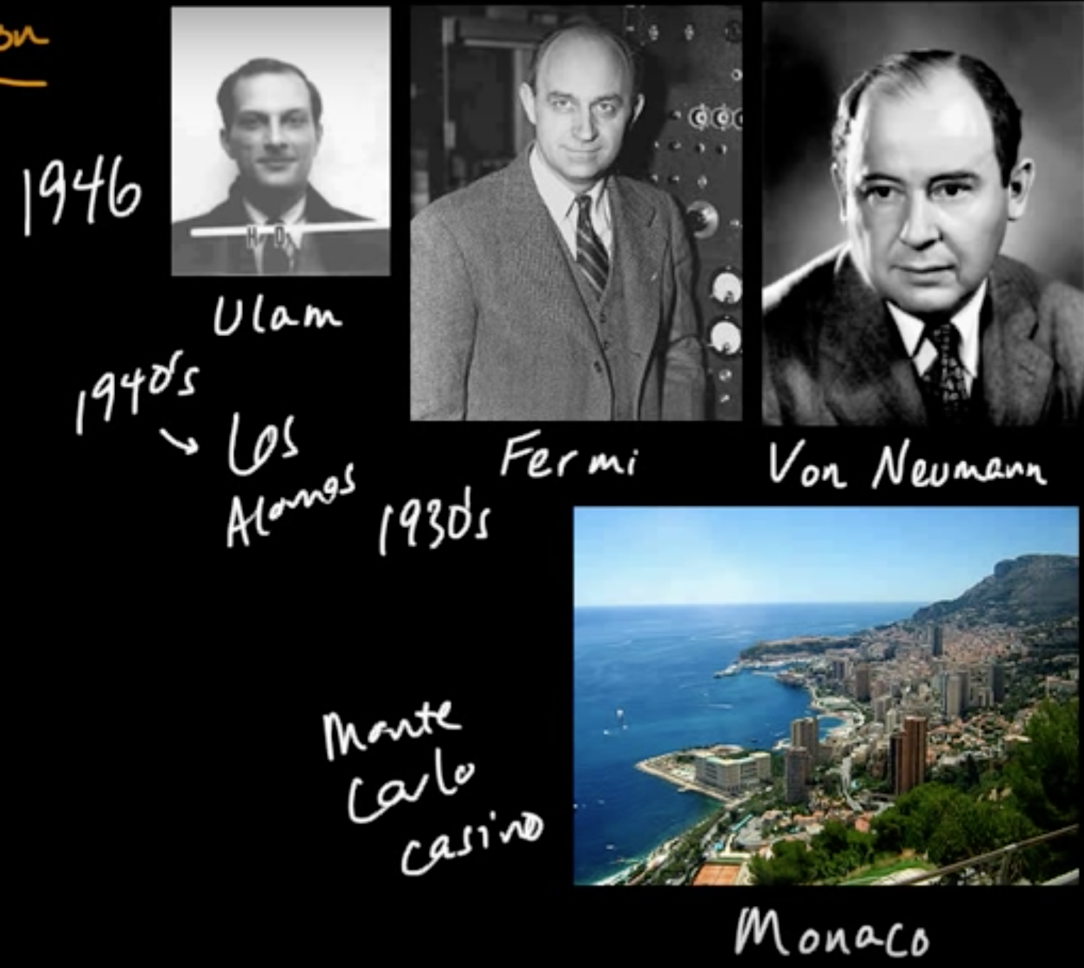
(ML 17.2) Monte Carlo methods - A little history

(ML 17.3) Monte Carlo approximation

Goal. Aprroximate $\mathbb{E}(f(X))$, when intractable to compute exactly.

Definition (Monte Carlo estimator). If $X_1, \ldots, X_n \sim p$, iid, then

is a (basic) Monte Carlo estimator of $\mathbb{E}(f(X))$ where $X \sim p$. (sample mean)

Remark
(1) $\mathbb{E}(\hat{\mu}_n) = \mathbb{E}(f(X))$ (i.e. $\hat{\mu}_n$ is an unbiased estimator)
(2) $\hat{\mu}_n \rightarrow^{\rm P} \mathbb{E}(f(X))$ as $n \rightarrow \infty$ $\Rightarrow$ consistenct estimator (assuming $\sigma^2(f(X))< \infty$) (i.e. $\forall \varepsilon >0, P(\vert \hat{\mu}_n - \mathbb{E}(f(X)) \vert < \varepsilon) \rightarrow 1$)
(3) $\sigma^2(\hat{\mu}_n) = \frac{1}{n}\sigma^2(f(X)) \rightarrow 0 \Rightarrow$ converges at a rate of $\frac{1}{\sqrt{n}}$ (regardless of dimension of $X$).
${\rm MSE}(\hat{\mu}_n = {\rm bias}^2 + {\rm var}) = \frac{1}{n}\sigma^(f(X)) \rightarrow 0$.

(ML 17.4) Examples of Monte Carlo approximation

1. Area of Mandelbrot set (Gamelin)
2. Expected return (investment)

(ML 17.5) Importance sampling - introduction

It’s not a sampling method but an estimation technique!

It can be thought of as a variant of MC estimation.

Recall. MC estimation (by sample mean):

under the BIG assumtion that $X \sim p$ and $X_i \sim p$.

Can we do something similar by drawing samples from an alternative distribution $q$?

Yes, and in some cases you can do much much better!

Density $p$ case.

holds for all pdf $q$ with respect to wchi $q$ is absolutely continuous, i.e., $p(x) = 0$ whenever $q(x)= 0$.

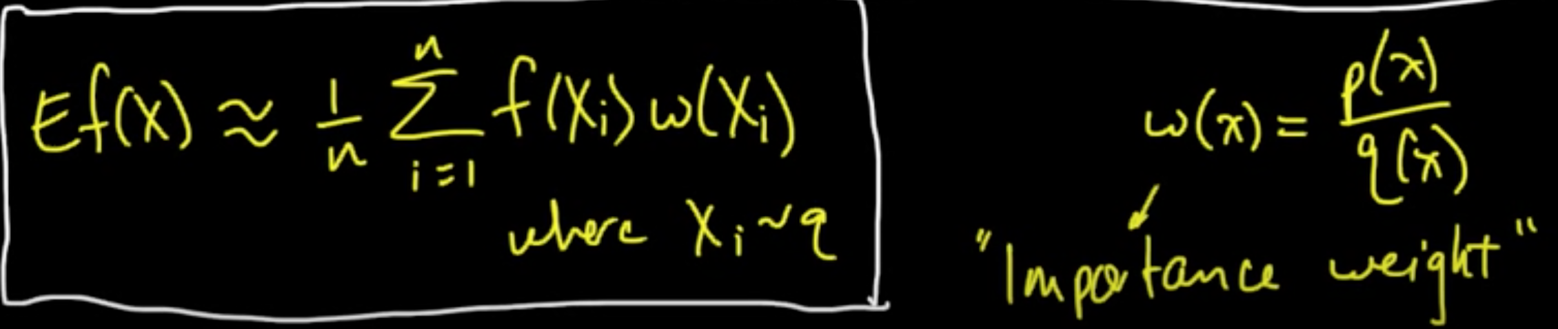
(ML 17.6) Importance sampling - intuition

What makes a good/bad choice of the proposal distrubution $q$?

To be added..