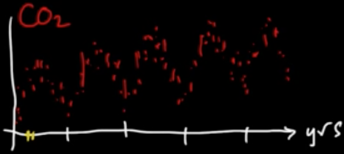
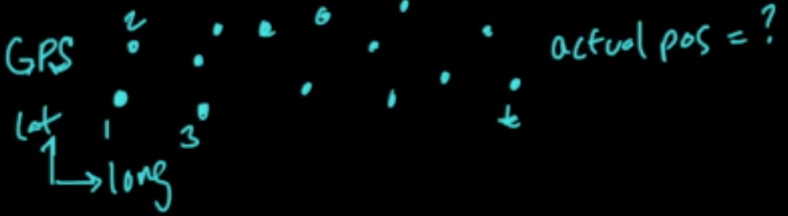
(ML 12.1) Model selection - introduction and examples

“Model” selection really means “complexity” selection!

Here, complexity $\approx$ flexibility to fit/explain data

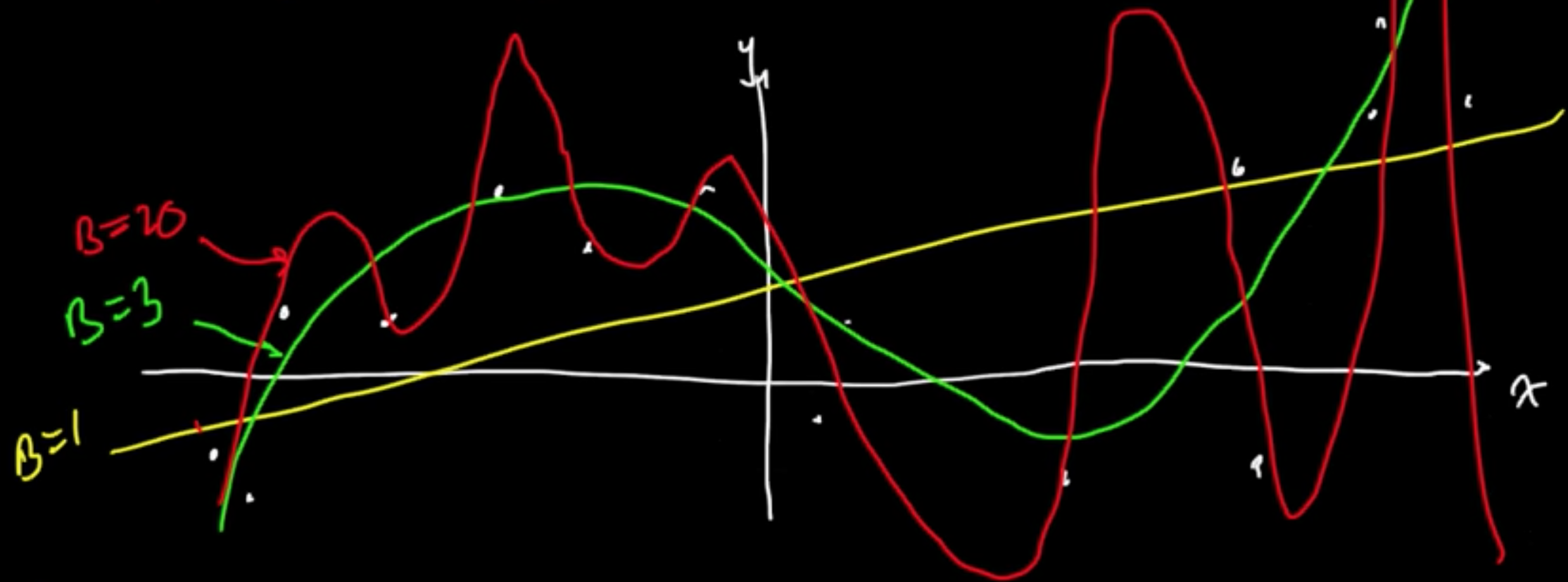
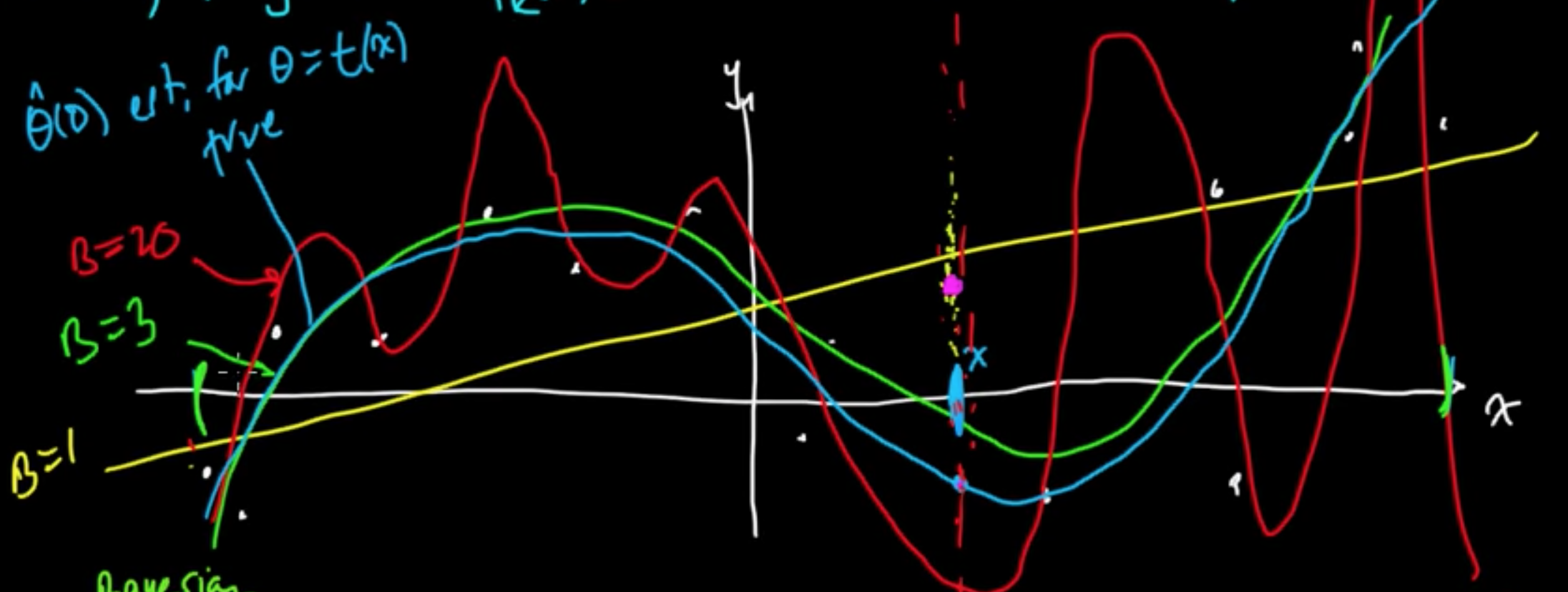
Example (Linaer regression with MLE for $w$) $f(x) = w^T\varphi(x)$
Given data $x \in \mathbb{R}$, consider polynomial basis $\varphi(x) = x^k$, $\varphi = (\varphi_0, \varphi_1, \ldots, \varphi_B)$

Turns out $B =$ “complexity parameter”

Example (Bayesia linear regression or MAP)

Example ($k$NN)

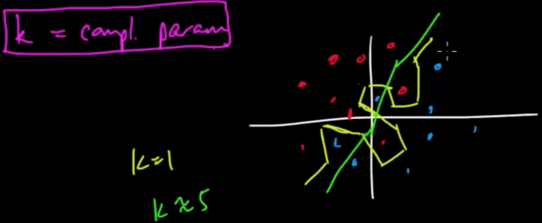
$k$ “controls” decesion boundaties.

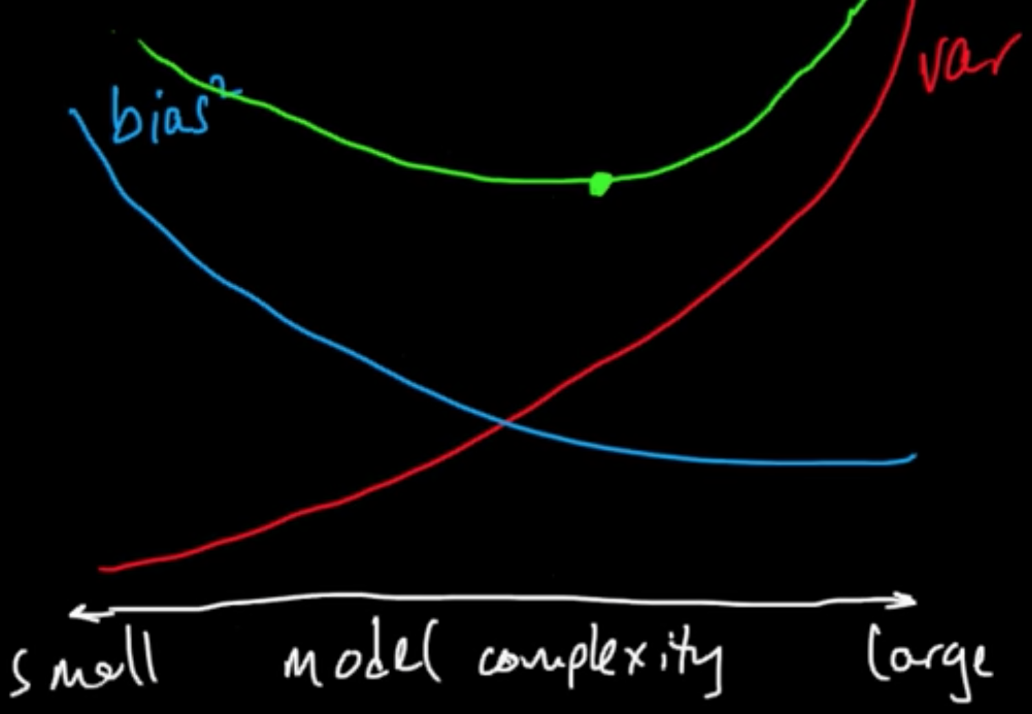
(ML 12.2) Bias-variance in model selection

Bias-variance trade-off, as they say.
MSE $=$ bias$^2 +$ var
Can do the same for intervals: $\int$MSE $=$ $\int$bias$^2 +$ $\int$var
(only applies for square loss)

(ML 12.3) Model complexity parameters

Complexitycontrolling parameters

• not parameters used to fit the data
• In Bayesian models, tend to be “hyperparameters” (i.e. parameters of the prior)

(ML 12.4) Bayesian model selection

«««< HEAD Bayesian Model Averaging (BMA) (just being fully Bayesian) ||||||| merged common ancestors —

(ML 14.1) Markov models - motivating examples

======= «««< HEAD «««< HEAD Bayesian Model Averaging (BMA) (just being fully Bayesian) ||||||| merged common ancestors —

(ML 14.1) Markov models - motivating examples

======= Bayesian Model Averaging (BMA) (just being fully Bayesian)

notes master

$p(y\vert x, \theta, m)$ where $\theta$ and $m$ are random variables

$p(y\vert x, D) = \inf p(y\vert x, \theta, m)p(m\vert x, D)dm$

where $p(y\vert x, D, m) = \int p(y\vert x, \theta, m)p(\theta \vert D, m)d\theta$

Alternative: “Type II MAP$^\star$”

«««< HEAD $p(y\vert x, D) \approx p(y\vert x, D, m^*)$ where $m^* \in \arg\max_mp(m\vert D)$ ||||||| merged common ancestors

======= «««< HEAD $p(y\vert x, D) \approx p(y\vert x, D, m^*)$ where $m^* \in \arg\max_mp(m\vert D)$

$p(m\vert D) \propto p(D\vert m)p(m)$

cf. Type II ML/Evidence Approximation/Empirical Bayes : ||||||| merged common ancestors

======= $p(y\vert x, D) \approx p(y\vert x, D, m^*)$ where $m^* \in \arg\max_mp(m\vert D)$

notes master

«««< HEAD $p(m\vert D) \propto p(D\vert m)p(m)$ ||||||| merged common ancestors (Sequential) Data: $D = (x_1, \ldots, x_n)$.
Model data as random variables: $X_1, \ldots, X_n$

• iid? No
• Everything depends on everything else. $\leadsto$ intractable problem

• $X_t$ depends on $X_{t-1}, X_{t-2}, \ldots, X_{t-m}$ for fixed $m$

  «««< HEAD $p(y\vert x, D) \approx p(y\vert x, D, m^*)$ where $m^* \in \arg\max_mp(D\vert m)$ ||||||| merged common ancestors (Sequential) Data: $D = (x_1, \ldots, x_n)$.
  Model data as random variables: $X_1, \ldots, X_n$

• iid? No
• Everything depends on everything else. $\leadsto$ intractable problem

• $X_t$ depends on $X_{t-1}, X_{t-2}, \ldots, X_{t-m}$ for fixed $m$

  $p(m\vert D) \propto p(D\vert m)p(m)$

  notes master

«««< HEAD cf. Type II ML/Evidence Approximation/Empirical Bayes : ||||||| merged common ancestors The simplest case $m=1$ (for the last line) leads to the notion of MArkov chain ======= «««< HEAD where $p(D\vert m)$ is called the marginal likelihood ||||||| merged common ancestors The simplest case $m=1$ (for the last line) leads to the notion of MArkov chain ======= cf. Type II ML/Evidence Approximation/Empirical Bayes :

notes master

$p(y\vert x, D) \approx p(y\vert x, D, m^*)$ where $m^* \in \arg\max_mp(D\vert m)$

«««< HEAD where $p(D\vert m)$ is called the marginal likelihood ||||||| merged common ancestors

(ML 14.2) (ML 14.3) Markov chains (discrete-time)

======= «««< HEAD

(ML 12.5) (ML 12.4) (ML 12.5) Cross-validation

||||||| merged common ancestors

(ML 14.2) (ML 14.3) Markov chains (discrete-time)

======= where $p(D\vert m)$ is called the marginal likelihood

notes

master

«««< HEAD

(ML 14.1) Markov models - motivating examples

||||||| merged common ancestors —

«««< HEAD

(ML 12.5) (ML 12.6) (ML 12.7) Cross-validation

||||||| merged common ancestors

(ML 15.1) Newton’s method (for optimization) - intuition

2nd order method!

(Gradient descent $x_{t+1} = x_t - \alpha_t \nabla f(x_t)$ : 1st order method)

Analogy (1D).

(ML 14.1) Markov models - motivating examples

======= Bayesian Model Averaging (BMA) (just being fully Bayesian)

notes

$p(y\vert x, \theta, m)$ where $\theta$ and $m$ are random variables

$p(y\vert x, D) = \inf p(y\vert x, \theta, m)p(m\vert x, D)dm$ ||||||| merged common ancestors

(ML 15.1) Newton’s method (for optimization) - intuition

2nd order method!

(Gradient descent $x_{t+1} = x_t - \alpha_t \nabla f(x_t)$ : 1st order method)

Analogy (1D).

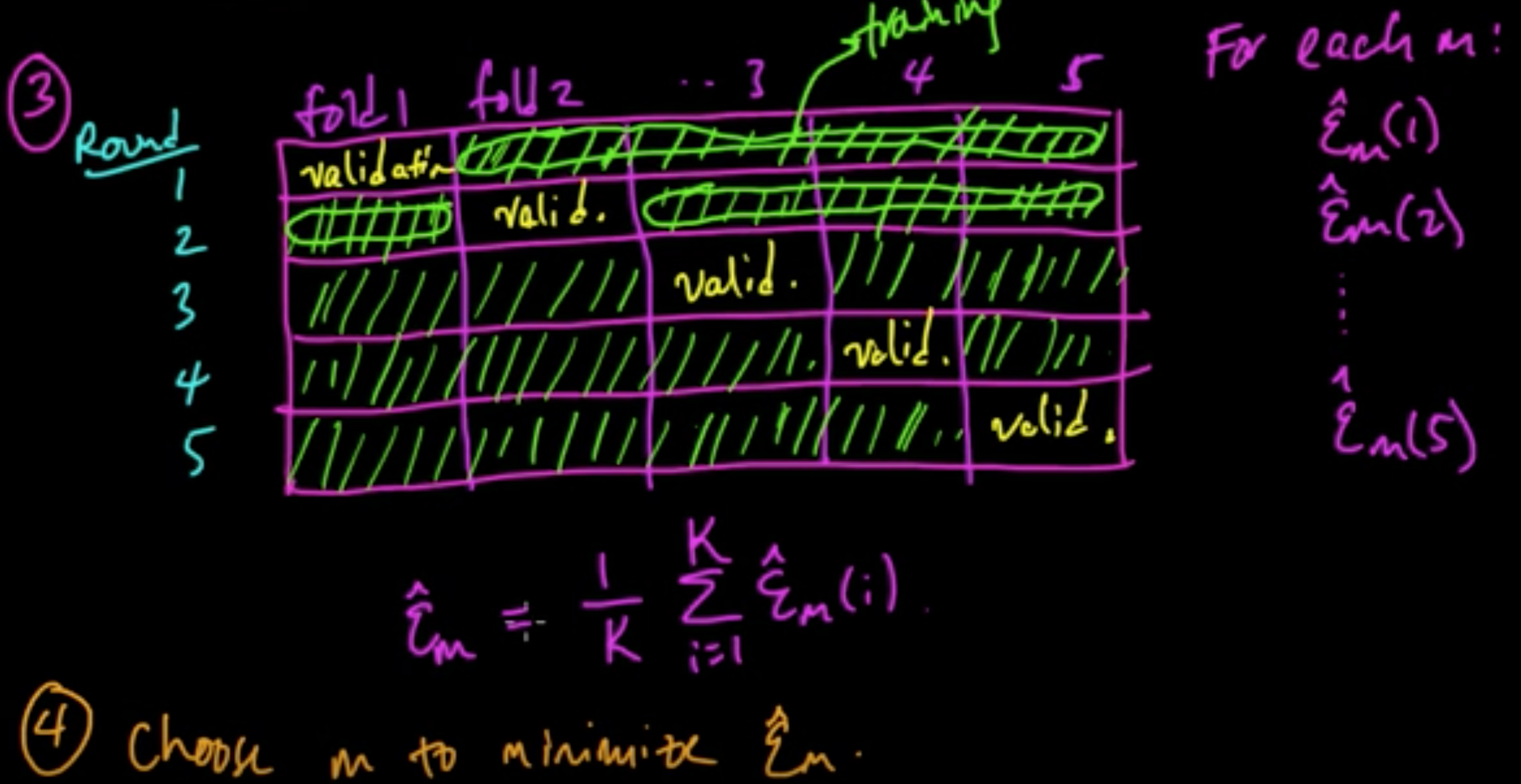
(ML 12.5) (ML 12.6) (ML 12.7) Cross-validation

notes master

«««< HEAD Data: $D = ((x_1, y_1), \ldots, (x_n, y_n))$ iid
Models: $m \in \{1, \ldots, C\}$
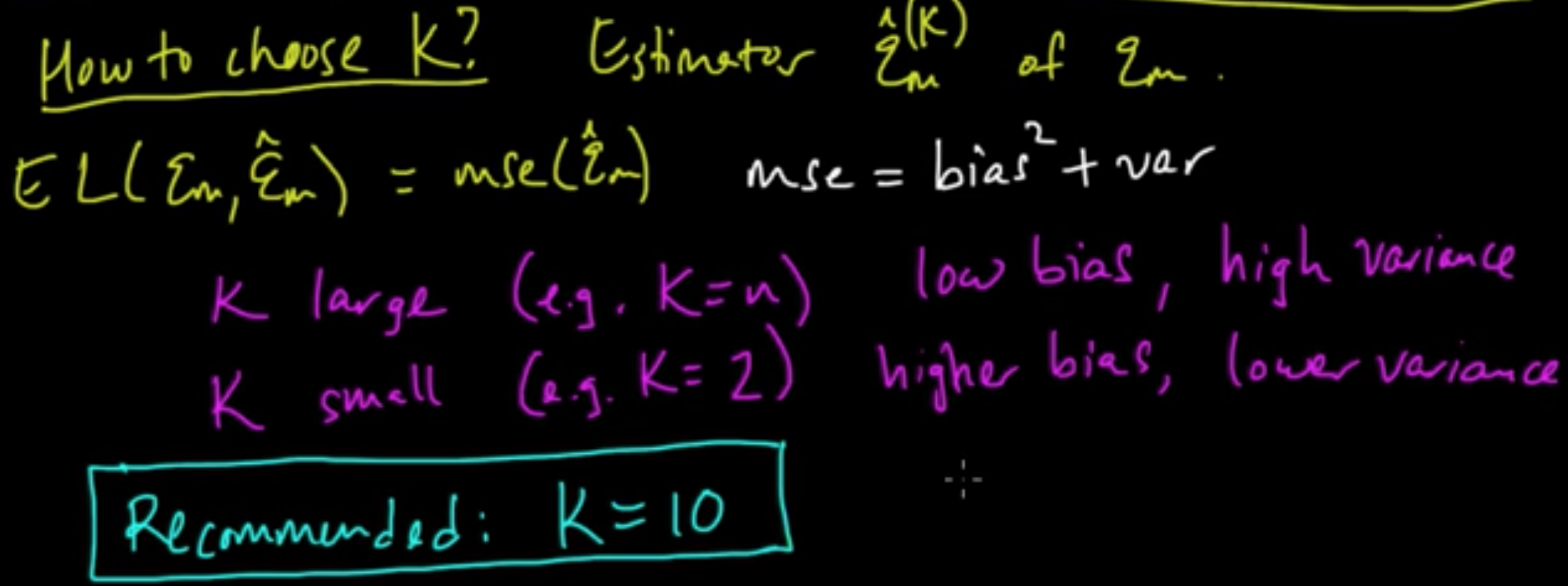
Error: $\varepsilon_m = {\rm EL}(Y, f_m(X))$ where $(X, Y) \sim p$ (true unknown distribution)

A. Validation ||||||| merged common ancestors

• zero-finding: $x_{t+1} = x_t - \frac{f(x_t)}{f’(x_t)}$

======= «««< HEAD where $p(y\vert x, D, m) = \int p(y\vert x, \theta, m)p(\theta \vert D, m)d\theta$ ||||||| merged common ancestors

• zero-finding: $x_{t+1} = x_t - \frac{f(x_t)}{f’(x_t)}$

  Data: $D = ((x_1, y_1), \ldots, (x_n, y_n))$ iid
  Models: $m \in \{1, \ldots, C\}$
  Error: $\varepsilon_m = {\rm EL}(Y, f_m(X))$ where $(X, Y) \sim p$ (true unknown distribution)

  notes

«««< HEAD Alternative: “Type II MAP$^\star$” ||||||| merged common ancestors

master

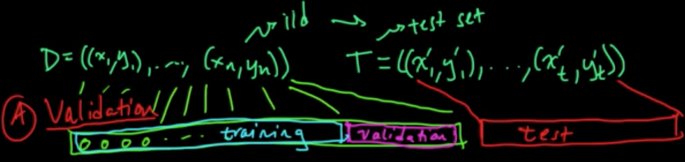
======= A. Validation

notes

«««< HEAD $p(y\vert x, D) \approx p(y\vert x, D, m^*)$ where $m^* \in \arg\max_mp(m\vert D)$

$p(m\vert D) \propto p(D\vert m)p(m)$

cf. Type II ML/Evidence Approximation/Empirical Bayes :

$p(y\vert x, D) \approx p(y\vert x, D, m^*)$ where $m^* \in \arg\max_mp(D\vert m)$

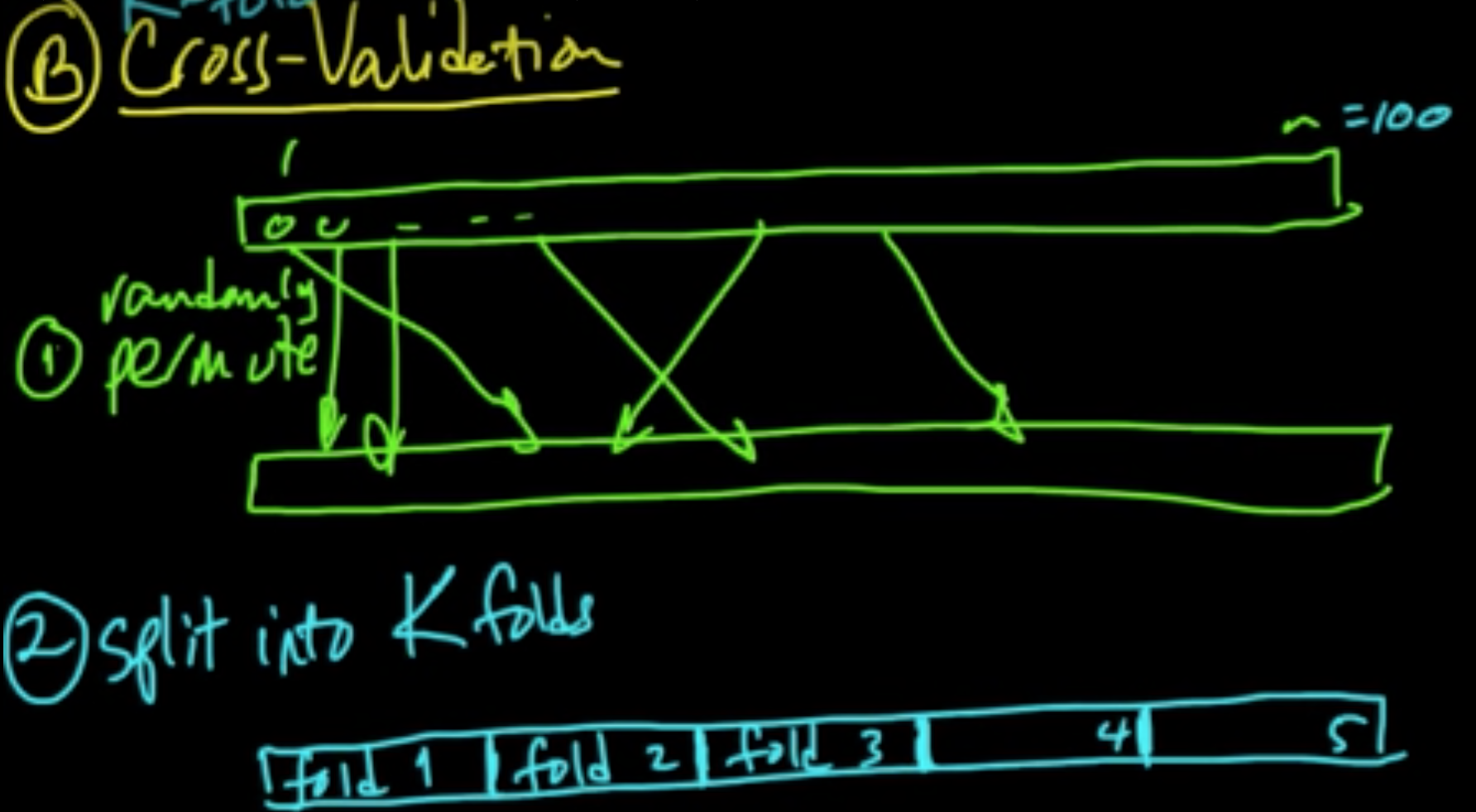
«««< HEAD B. Cross-validation ||||||| merged common ancestors

• min./maximizing: $x_{t+1} = x_t - \frac{f’(x_t)}{f’‘(x_t)}$

======= where $p(D\vert m)$ is called the marginal likelihood

(ML 12.5) (ML 12.6) (ML 12.7) Cross-validation

Data: $D = ((x_1, y_1), \ldots, (x_n, y_n))$ iid
Models: $m \in \{1, \ldots, C\}$
Error: $\varepsilon_m = {\rm EL}(Y, f_m(X))$ where $(X, Y) \sim p$ (true unknown distribution)

A. Validation ||||||| merged common ancestors

• min./maximizing: $x_{t+1} = x_t - \frac{f’(x_t)}{f’‘(x_t)}$

master

«««< HEAD ||||||| merged common ancestors

(ML 15.2) Newton’s method (for optimization) in multiple dimensions

Idea: “Make a 2nd order approximation and minimize tha.”

Let $f: \mathbb{R}^n \rightarrow \mathbb{R}$ be (sufficiently) smooth.

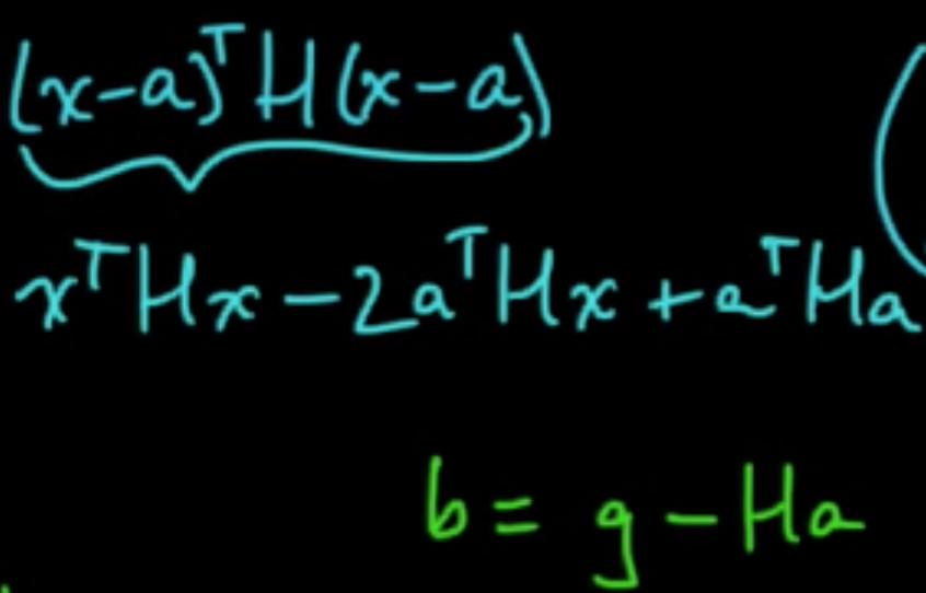
Taylor’s theorem: for $x$ near a, letting $g = \nabla f(a)$ and $H = \nabla^2f(a) = \left(\frac{\partial^2}{\partial x_i \partial x_j}f(a)\right)_{ij}$,

=======

(ML 15.2) Newton’s method (for optimization) in multiple dimensions

Idea: “Make a 2nd order approximation and minimize tha.”

Let $f: \mathbb{R}^n \rightarrow \mathbb{R}$ be (sufficiently) smooth.

Taylor’s theorem: for $x$ near a, letting $g = \nabla f(a)$ and $H = \nabla^2f(a) = \left(\frac{\partial^2}{\partial x_i \partial x_j}f(a)\right)_{ij}$,

======= B. Cross-validation

notes master

<<<<<<< HEAD ||||||| merged common ancestors ======= <<<<<<< HEAD ||||||| merged common ancestors ======= >>>>>>> notes >>>>>>> master

(5) Retrain using $m^*$ on all of $D$.

«««< HEAD C. LOOCV (Leave-One-Out CV) $k = n$ ||||||| merged common ancestors Minimize: $0 = \nabla q = Hx + b \Rightarrow x = -H^{-1}b = a -H^{-1}g$

Critical to check: $\nabla^2 q = H$ $\Rightarrow$ minimum if $H$ is PSD.

Algorithm.

• Initialize $x \in \mathbb{R}^n$
• Iterate: $x_{t+1} = x_t - H^{-1}g$ where $g = \nabla f(x_t), H = \nabla^2 f(x_t)$

Issues.

1. $H$ may fail to be PSD. (Option: switch gradient descent. A smart way to do it: Levenberg–Marquardt algorithm)
2. Rather than invert $H$, sove $Hy = g$ for $y$, then use $x_{t+1} = x_t - y$. (More robust approach)
3. $x_{t+1} = x_t - \alpha_t y$. (small “step size” $\alpha_t>0$)

(ML 16.6) Gaussian mixture model (Mixture of Gaussians)

======= «««< HEAD B. Cross-validation ||||||| merged common ancestors Minimize: $0 = \nabla q = Hx + b \Rightarrow x = -H^{-1}b = a -H^{-1}g$

Critical to check: $\nabla^2 q = H$ $\Rightarrow$ minimum if $H$ is PSD.

Algorithm.

• Initialize $x \in \mathbb{R}^n$
• Iterate: $x_{t+1} = x_t - H^{-1}g$ where $g = \nabla f(x_t), H = \nabla^2 f(x_t)$

Issues.

1. $H$ may fail to be PSD. (Option: switch gradient descent. A smart way to do it: Levenberg–Marquardt algorithm)
2. Rather than invert $H$, sove $Hy = g$ for $y$, then use $x_{t+1} = x_t - y$. (More robust approach)
3. $x_{t+1} = x_t - \alpha_t y$. (small “step size” $\alpha_t>0$)

(ML 16.6) Gaussian mixture model (Mixture of Gaussians)

master

«««< HEAD D. Random Subsamples ||||||| merged common ancestors ======= ======= C. LOOCV (Leave-One-Out CV) $k = n$

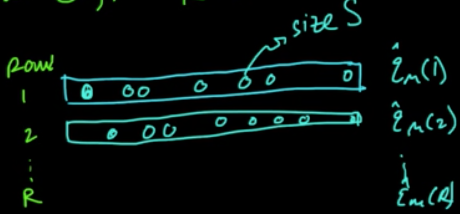
D. Random Subsamples

notes master

<<<<<<< HEAD ||||||| merged common ancestors ======= <<<<<<< HEAD ||||||| merged common ancestors ======= >>>>>>> notes >>>>>>> master

«««< HEAD ||||||| merged common ancestors

«««< HEAD ||||||| merged common ancestors $Z \in \{e_1, \ldots, e_m\}$, standard vectors in $\mathbb{R}^m$ ($Z$ is “latent” variable)
$P(Z = e)k = \alpha_k$
Given $Z = e_k$,
$X \sim N(\mu_k, C_k)$
where $\mu_1, \ldots, \mu_m \in \mathbb{R}^d$ and $C_1, \ldots, C_m$ $d\times d$ cov. matrices.

======= $Z \in \{e_1, \ldots, e_m\}$, standard vectors in $\mathbb{R}^m$ ($Z$ is “latent” variable)
$P(Z = e)k = \alpha_k$
Given $Z = e_k$,
$X \sim N(\mu_k, C_k)$
where $\mu_1, \ldots, \mu_m \in \mathbb{R}^d$ and $C_1, \ldots, C_m$ $d\times d$ cov. matrices.

=======

notes master

<<<<<<< HEAD ||||||| merged common ancestors ======= <<<<<<< HEAD ||||||| merged common ancestors ======= >>>>>>> notes

(5) Retrain using $m^*$ on all of $D$.

«««< HEAD C. LOOCV (Leave-One-Out CV) $k = n$

D. Random Subsamples

>>>>>>> master

«««< HEAD ||||||| merged common ancestors Marginal distribution:
$\begin{aligned} p(x) & = \sum_z p(x\vert z)p(z) \\ & = \sum_{k=1}^m P(Z = e_k) P(x \vert Z = e_k) \\ & = \sum_{k=1}^m \alpha_k N(x \vert \mu_k, C_k) \end{aligned}$

The $\alpha_k$ are called the mixing coefficients.

Joint distribution:

where $z = (z_1, \ldots, z_m)$

On the other hand,

Note that $P(Z = e_k \vert x) = \mathbb{E}(I(Z=e_k)\vert X=x)$.

(ML 17.1) Sampling methods - why sampling, pros and cons

Why is sampling so powerful and useful?

• For approximating expectations ($\leadsto$ estimate statistics / posterior infernce i.e. computing probability)
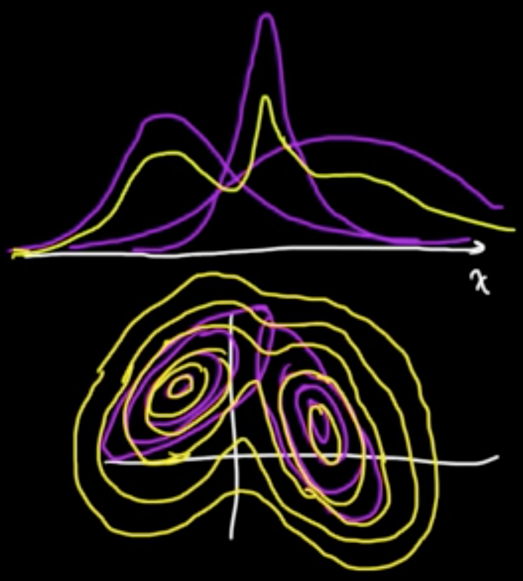
• For visualization of typical draws from a distribution of interest

Why expectations?

• Any probability is an expectation: $P(X \in A) = E(I_{X \in A})$.
• Approximation is needed for intractable sums/integrals (can be expressed as expectations)

Pros.

• Easy (both to implement and to understand)
• General purpose (widely applicable)

Cons.

• Too easy (used inappropriately)
• Slow (usually need lots of samples)
• Getting “good” samples may be dificult
• Difficult to assess the performance of methods (e.g. MCMC)

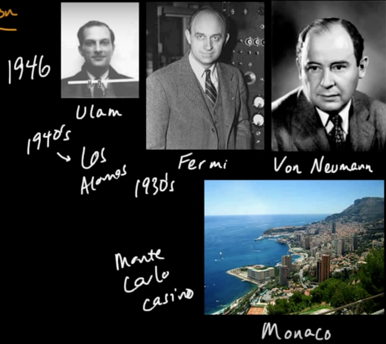
(ML 17.2) Monte Carlo methods - A little history

(ML 17.3) Monte Carlo approximation

Goal. Aprroximate $\mathbb{E}(f(X))$, when intractable to compute exactly.

Definition (Monte Carlo estimator). If $X_1, \ldots, X_n \sim p$, iid, then

is a (basic) Monte Carlo estimator of $\mathbb{E}(f(X))$ where $X \sim p$. (sample mean)

Remark
(1) $\mathbb{E}(\hat{\mu}_n) = \mathbb{E}(f(X))$ (i.e. $\hat{\mu}_n$ is an unbiased estimator)
(2) $\hat{\mu}_n \rightarrow^{\rm P} \mathbb{E}(f(X))$ as $n \rightarrow \infty$ $\Rightarrow$ consistenct estimator (assuming $\sigma^2(f(X))< \infty$) (i.e. $\forall \varepsilon >0, P(\vert \hat{\mu}_n - \mathbb{E}(f(X)) \vert < \varepsilon) \rightarrow 1$)
(3) $\sigma^2(\hat{\mu}_n) = \frac{1}{n}\sigma^(f(X)) \rightsrrow 0 \Rightarrow$ converges at a rate of $\frac{1}{\sqrt{n}}$ (regardless of dimension of $X$).
${\rm MSE}(\hat{\mu}_n = {\rm bias}^2 + {\rm var}) = \frac{1}{n}\sigma^(f(X)) \rightarrow 0$.

(ML 17.4) Examples of Monte Carlo approximation

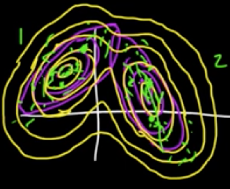
1. Area of Mandelbrot set (Gamelin)
2. Expected return (investment)

(ML 17.5) Importance sampling - introduction

It’s not a sampling method but an estimation technique!

It can be thought of as a variant of MC estimation.

Recall. MC estimation (by sample mean):

under the BIG assumtion that $X \sim p$ and $X_i \sim p$.

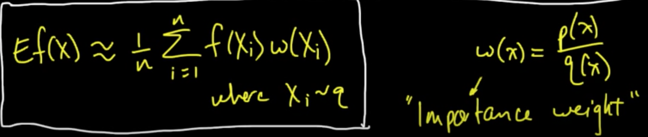
Can we do something similar by drawing samples from an alternative distribution $q$?

Yes, and in some cases you can do much much better!

Density $p$ case.

holds for all pdf $q$ with respect to wchi $q$ is absolutely continuous, i.e., $p(x) = 0$ whenever $q(x)= 0$.

(ML 17.6) Importance sampling - intuition

What makes a good/bad choice of the proposal distrubution $q$?

To be added..

======= ||||||| merged common ancestors Marginal distribution:
$\begin{aligned} p(x) & = \sum_z p(x\vert z)p(z) \\ & = \sum_{k=1}^m P(Z = e_k) P(x \vert Z = e_k) \\ & = \sum_{k=1}^m \alpha_k N(x \vert \mu_k, C_k) \end{aligned}$

The $\alpha_k$ are called the mixing coefficients.

Joint distribution:

where $z = (z_1, \ldots, z_m)$

On the other hand,

Note that $P(Z = e_k \vert x) = \mathbb{E}(I(Z=e_k)\vert X=x)$.

(ML 17.1) Sampling methods - why sampling, pros and cons

Why is sampling so powerful and useful?

• For approximating expectations ($\leadsto$ estimate statistics / posterior infernce i.e. computing probability)
• For visualization of typical draws from a distribution of interest

Why expectations?

• Any probability is an expectation: $P(X \in A) = E(I_{X \in A})$.
• Approximation is needed for intractable sums/integrals (can be expressed as expectations)

Pros.

• Easy (both to implement and to understand)
• General purpose (widely applicable)

Cons.

• Too easy (used inappropriately)
• Slow (usually need lots of samples)
• Getting “good” samples may be dificult
• Difficult to assess the performance of methods (e.g. MCMC)

(ML 17.2) Monte Carlo methods - A little history

(ML 17.3) Monte Carlo approximation

Goal. Aprroximate $\mathbb{E}(f(X))$, when intractable to compute exactly.

Definition (Monte Carlo estimator). If $X_1, \ldots, X_n \sim p$, iid, then

is a (basic) Monte Carlo estimator of $\mathbb{E}(f(X))$ where $X \sim p$. (sample mean)

Remark
(1) $\mathbb{E}(\hat{\mu}_n) = \mathbb{E}(f(X))$ (i.e. $\hat{\mu}_n$ is an unbiased estimator)
(2) $\hat{\mu}_n \rightarrow^{\rm P} \mathbb{E}(f(X))$ as $n \rightarrow \infty$ $\Rightarrow$ consistenct estimator (assuming $\sigma^2(f(X))< \infty$) (i.e. $\forall \varepsilon >0, P(\vert \hat{\mu}_n - \mathbb{E}(f(X)) \vert < \varepsilon) \rightarrow 1$)
(3) $\sigma^2(\hat{\mu}_n) = \frac{1}{n}\sigma^(f(X)) \rightsrrow 0 \Rightarrow$ converges at a rate of $\frac{1}{\sqrt{n}}$ (regardless of dimension of $X$).
${\rm MSE}(\hat{\mu}_n = {\rm bias}^2 + {\rm var}) = \frac{1}{n}\sigma^(f(X)) \rightarrow 0$.

(ML 17.4) Examples of Monte Carlo approximation

1. Area of Mandelbrot set (Gamelin)
2. Expected return (investment)

(ML 17.5) Importance sampling - introduction

It’s not a sampling method but an estimation technique!

It can be thought of as a variant of MC estimation.

Recall. MC estimation (by sample mean):

under the BIG assumtion that $X \sim p$ and $X_i \sim p$.

Can we do something similar by drawing samples from an alternative distribution $q$?

Yes, and in some cases you can do much much better!

Density $p$ case.

holds for all pdf $q$ with respect to wchi $q$ is absolutely continuous, i.e., $p(x) = 0$ whenever $q(x)= 0$.

(ML 17.6) Importance sampling - intuition

What makes a good/bad choice of the proposal distrubution $q$?

To be added..

=======

notes master —