
Notes on Machine Learning 8: Naive Bayes
by 장승환
(ML 8.1) Naive Bayes classification
Naive Bayes is a family of models that is not necessarily a “Bayesian” method!
Setup: Given data $D = ((x^{(1)}, y_1), \ldots, (x^{(n)}, y_n))$
with $x^{(i)} = (x_1^{(1)}, \ldots, x_1^{(d)}) \in \mathbb{R}^d$ and $y_i \in \mathcal{Y} = \{1, \ldots, m\}$.
Assume a family of joint distributions $p_\theta$ such that
Let $(X^{(1)}, Y_1) , \ldots, (X^{(n)}, Y_n) \sim p_\theta$, iid, for some $\theta$.
(If $(X, Y) \sim p_\theta$, then $X_1, \ldots, X_d$ are (conditionally) independent given $Y$.)
Goal: For new $x \in \mathbb{R}^d$, pridict it’s $y$.
Algorithm:
- Estimate $\hat{\theta}$ from $D$.
- Then compute
(ML 8.2) More about Naive Bayes
Assume that $(X, Y) \sim p_\theta$ with $Y \in \mathscr{Y} \in \{1, \ldots, m\}.$
How to choose $p_\theta$?
- $p_\theta(y) = p_\theta(Y = y) := \pi$ with $\pi = (\pi_1, \ldots, \pi_m)$.
- $p_\theta(x_i\vert y) = p_\theta(X_i = x \vert Y = y)$
$\theta =$ (all parameters of the distributions)
If $X_i \in \{1, \ldots, N\}$ then e.g. $p_\theta(x_i\vert y) := q(x_i, y)$.
If $X_i \in \{1, 2, \ldots\}$ then e.g. Poisson or Geometric or whatever.
If $X_i \in \mathbb{R}$ then e.g. Gaussian, Gamma or whatever.
How to estimate $\theta$?
MLE, or MAP (assuming priro on $\theta$)
Another option: “Bayesian” naive Nayes
Why make conditional independence assumption?
Can estimate $\theta$ more accurately with less data.
“Wrong but simple model can be better than correct but complicated model!”
(ML 8.3) (ML 8.4) Bayesian Naive Bayes
Assume that $(X, y) \sim p(x,y\vert \theta)$.
$D = ((x^{(1)}, y_1), \ldots, (x^{(n)},y))$ where
$x^{(i)}= (x_1^{(i)}, \ldots, x_d^{(i)})$ and the $j$-th feature $x_j^{(i)} \in A_j$
and $y \in \mathscr{Y} = \{1, \ldots, m\}$
$(X^{(1)}, Y_1), \ldots, (X^{(n)}, Y_n) \sim p(x,y\vert \theta)$ independent given $\theta = (\pi, \{r_jy\})$
Naive Bayes assumption says that the features are independent given the class & the parameter
- $p(y\vert \theta) = \pi(y)$ where $\pi = (\pi(1), \ldots, \pi(m))$
- $p(x_j\vert y, \theta) = P(X_J = x_j\vert Y=y, \theta) = r_{jy}(x_j)$
($\sum \pi(y)=1, \sum_{k \in A_j}r_{jy} \forall j, y$)
Let’s put some prior: a natural choice is Dirichlet.
(Dirichlet is a conjugate prior for categorical distribution.)
…
(ML 11.1) Estimators
Assume the data $D = (X_1, \ldots, X_n)$ are given as random variables.
Definition. A statistic is a random variable $S = f(D)$ that is a function of the data $D$.
Terminology. An estimator is a statistic intended to approximate a parameter governing the distribution of $D$.
Notation.
- $\hat{\theta}$ denotes an estimator of a parameter $\theta$.
- $\hat{\theta}_n$ emphasize (the dependence on) $n$
Example. $X_1, \ldots, X_n \sim N(\mu, \sigma^2)$ iid
(Sample mean) $\,\,$ $\hat{\mu} = \bar{X} = \frac{1}{n}\sum_{i=1}^nX_i$ $\,\,$ /cf. $\sigma^2 = \mathbb{E}((X - \mu)^2)$
(“Biased” sample variance) $\,\,$ $\hat{\sigma}^2 = \frac{1}{n}\sum_{i=1}^n(X_i -\bar{X})^2$
(“unbiased” sample variance) $\,\,$ $s^2 = \frac{1}{n-1}\sum_{i=1}^n(X_i -\bar{X})^2$
Definition.
- The bias of an estimator $\hat{\theta}$ is $\,$ ${\rm bias}(\hat{\theta}) = \mathbb{E}(\hat{\theta}) - \theta$.
- An estimator $\hat{\theta}$ is unbiased if $\,$ ${\rm bias}(\theta) = 0$.
Example.
- $\hat{\mu}$ is unbiased: $\mathbb{E}(\hat{\mu}) = \mathbb{E}(\frac{1}{n}\sum_{i=1}^nX_i) =\frac{1}{n}\sum \mathbb{E}(X_i) = \frac{1}{n}\sum \mu = \mu$
- $\hat{\sigma}^2$ is biased. (Exercise)
- $s^2$ is unbiased. (Exercise)
(ML 11.2) Decision theory terminology in different contexts
| General | Estimators | $^*$Regression/Classification |
| Decision rule $\delta$ | $^*$Estimator function $g$ | Prediction function $f$ |
| State $s$ (unknown) | Parameter $\theta$ (unknown) | Target value $Y$ (unknown) |
| $^*$Data $D$ (observed) | Data $D$ (observed) | Point $X$ (observed) |
| Action $a = \delta(D)$ | Estimator/Estimate $\hat{\theta}=g(D)$ | Prediction $\hat{Y} = f(X)$ |
| Loss $L(s, a)$ | Loss $L(\theta, \hat{\theta})$ | Loss $L(Y, \hat{Y})$ |
Example. (Estimators)
An estimator is a random rariable: $\hat{\mu} = \frac{1}{n} \sum_{i=1}^n X_i$.
An estimate is a number: $\hat{\mu} = \frac{1}{n} \sum_{i=1}^n x_i = 2.3$.
(In some situation, the procedure $g$ is refered to as an estimator!)
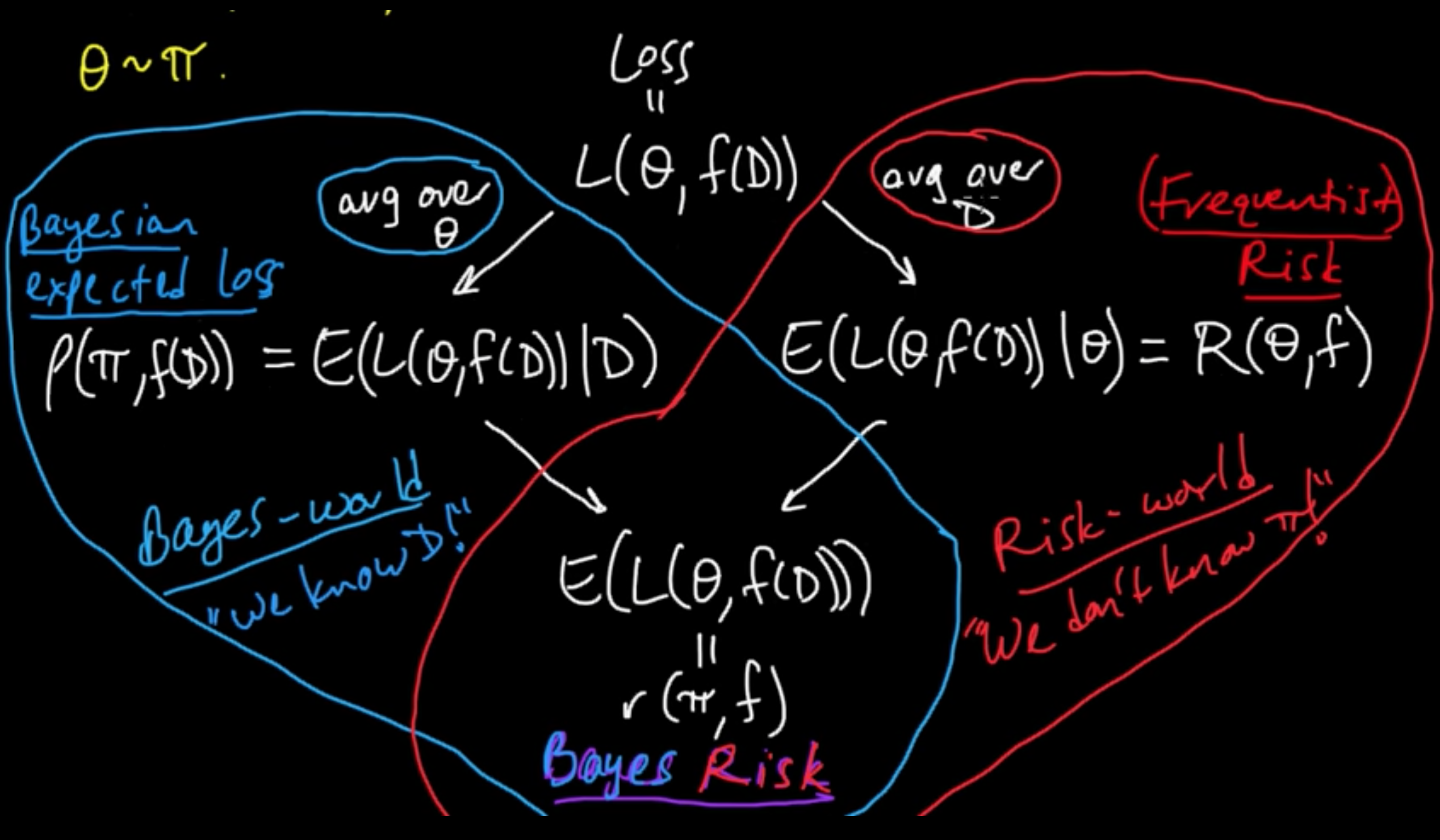
(ML 11.3) Frequentist risk, Bayesian expected loss, and Bayes risk
Loss and Risk. Exciting session to clear up all the mud!
Data: $\,$ $D = (X_1, \ldots, X_n)$, $D \sim p_\theta$
Parameter: $\,$ $\theta \sim \pi$ $\,$, i.e., the parameter $\theta$ is a random variable.
Estimator: $\,$ $\hat{\theta} = f(D) = \delta(D)$
Everything begins with : $\,\,\,\,\,$ Loss $=L(\theta, f(D))$.
We wanna minimize the loss but it’s an RV!
Two option to deal with it:
- Averaging over $\theta$ given the data : $E(L(\theta, f(D)) \vert D) =:\rho(\pi, f(D))$ Bayesian expected loss
- Averaging over the data given $\theta$ : $E(L(\theta, f(D)) \vert \theta) =: R(\theta, f)$ (Frequentist) risk
(ML 11.4) Choosing a decision rule - Bayesian and frequentist
How to choose $f$.
Bayesian: Assume $\pi$
Case 1. Know $D$. Choose $f(D)$ to minimize $\rho(\pi, f(D))$
Case 2. Don’t know $D$. Choose $f$ to minimize $r(\pi, f)$
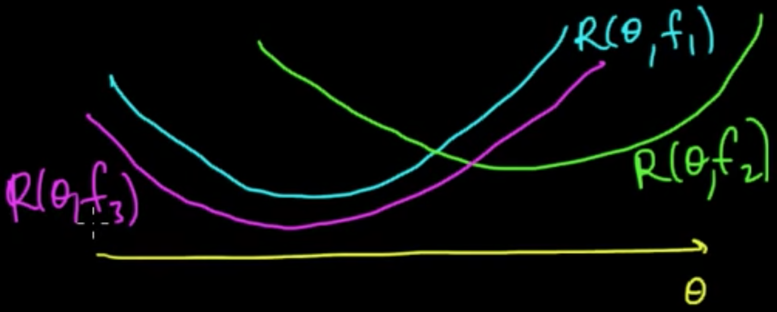
Frequentist: Introduce a furthere principle to guide your choice.
(a) Unbiasedness
(b) Admissibility
(c) Minimax
(d) Invariance
(ML 11.5) Bias-Variance decomposition (MSE $=$ bias$^2$ + var)
“A super impportant port of ML is what’s called model selection and a tool for model selection is the bias-variance decomposition.”
Almost trivial identity but extremely handy.
Definition. Let $D$ be random data. The MSE of an estimator $\hat{\theta} = f(D)$ for $\theta$ is
Put $\vert \theta$ emphasizing we’re not averagning over $\theta$ here (we don’t have a distribution over $\theta$). We’re just averaging over the data.
MSE$\theta$ is nothing but the risk $R(\theta, f)$ under square loss, i.e., when the loss function is the square of the deifference.
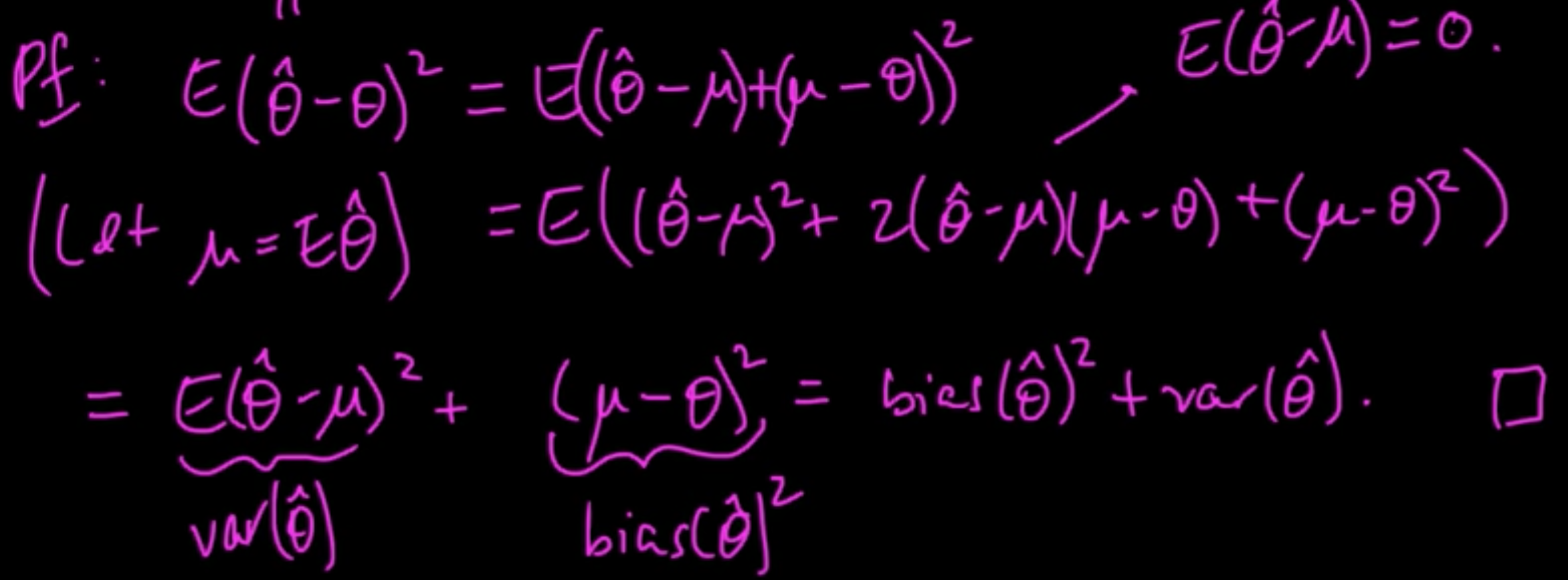
Recall. bias$(\hat{\theta}) = E(\theta) -\theta$.
Proposition. MSE$(\theta) = bias(\hat{\theta})^2 + {\rm var}(\hat{\theta})$
Proof:
Silly example. $X \sim N(\theta, 1)$ $\theta$ nonrandom & unknown $D = X
“Natural” estimate of $\theta$: $\delta_1(D) = X \leadsto$ bias$^2 = 0$, var$ = 1$, MSE$ =1$
“Silly” estimate of $\theta$: $\delta_0(D) = X \leadsto$ bias$^2 = \theta^2$, var$ = 0$, MSE$ = \theta^2$
cf. Shrinkage, Stein’s paradox
(ML 11.8) Bayesian decision theory
Terminology.(Informal)
- A generalized Bayes rule is a decision rule $\delta$ that minimizes $\rho(\pi, \delta(D))$ for each $D$.
- A Bayes rule minimizes is a decision rule $\delta$ that minimizes $r(\pi, \delta)$.
Remark
- GBR $\Rightarrow$ BR, but BR $\not\Rightarrow$ GBR.
- If $r(\pi, \delta) = \infty$ for all $\delta$, then anything is a BR, but a GBR still makes sense.
- On a set of $\pi$-measure $0$, BR is arbitrary bit GBR is still sensible.
Complete Class Theorems. Under mild conditions:
- Every GBR (for a proper $\pi$) is admissible;
- Every admissible decision rule is a GBR for some (possibly improper) $\pi$
Check out:
- Complete Class Theorems for the Simplest Empirical Bayes Decision Problems
- A Complete Class Theorem for Statistical Problems with Finite Sample Spaces
(ML 12.1) Model selection - introduction and examples
“Model” selection really means “complexity” selection!
Here, complexity $\approx$ flexibility to fit/explain data
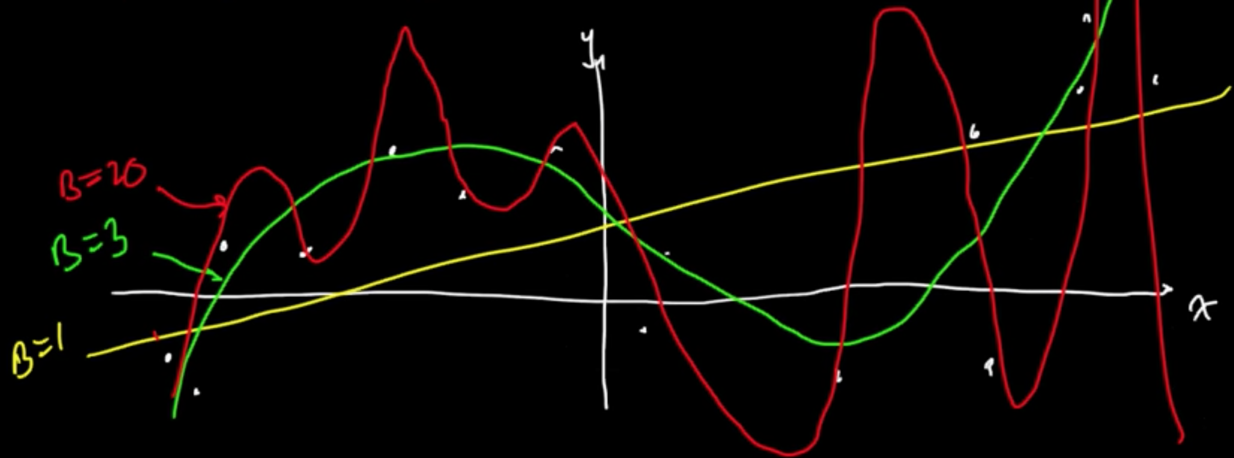
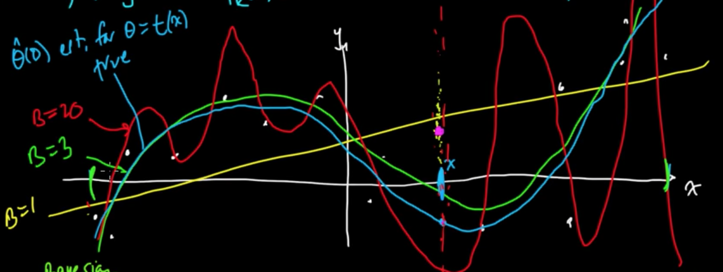
Example (Linaer regression with MLE for $w$) $f(x) = w^T\varphi(x)$
Given data $x \in \mathbb{R}$, consider polynomial basis $\varphi(x) = x^k$, $\varphi = (\varphi_0, \varphi_1, \ldots, \varphi_B)$
Turns out $B =$ “complexity parameter”
Example (Bayesia linear regression or MAP)

Example ($k$NN)
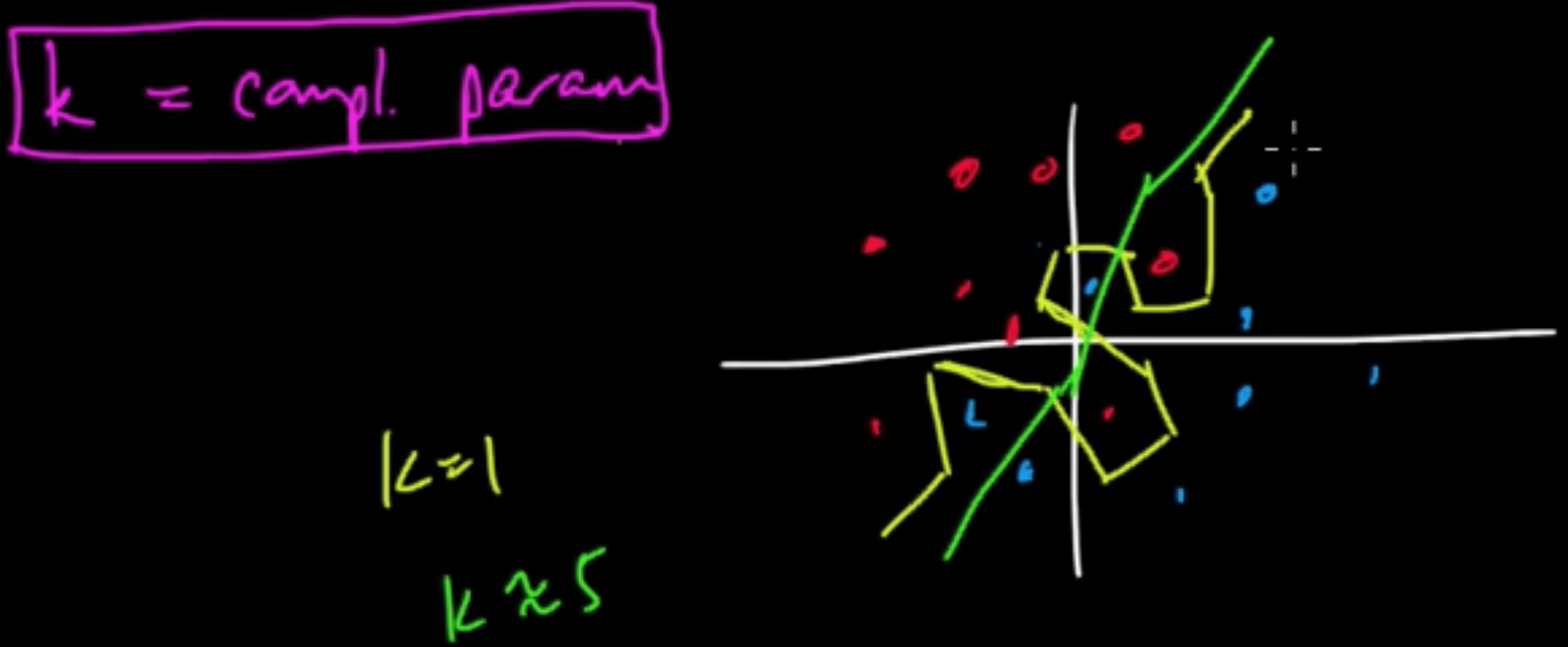
$k$ “controls” decesion boundaties.
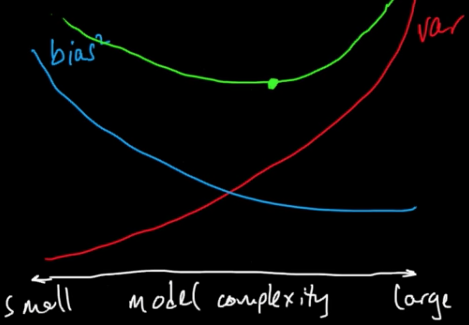
(ML 12.2) Bias-variance in model selection
Bias-variance trade-off, as they say.
MSE $=$ bias$^2 +$ var / $\in$MSE $=$ $\int$bias$^2 +$ $\int$var (only applies for square loss)
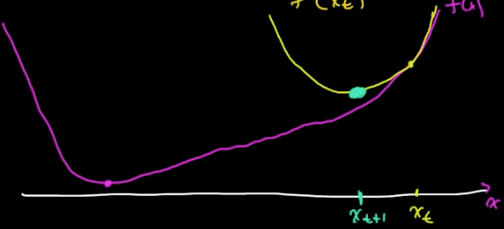
(ML 15.1) Newton’s method (for optimization) - intuition
2nd order method!
(Gradient descent $x_{t+1} = x_t - \alpha_t \nabla f(x_t)$ : 1st order method)
Analogy (1D).
- zero-finding: $x_{t+1} = x_t - \frac{f(x_t)}{f’(x_t)}$
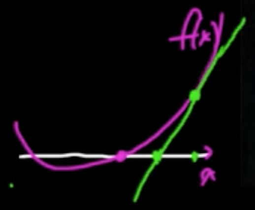
- min./maximizing: $x_{t+1} = x_t - \frac{f’(x_t)}{f’‘(x_t)}$
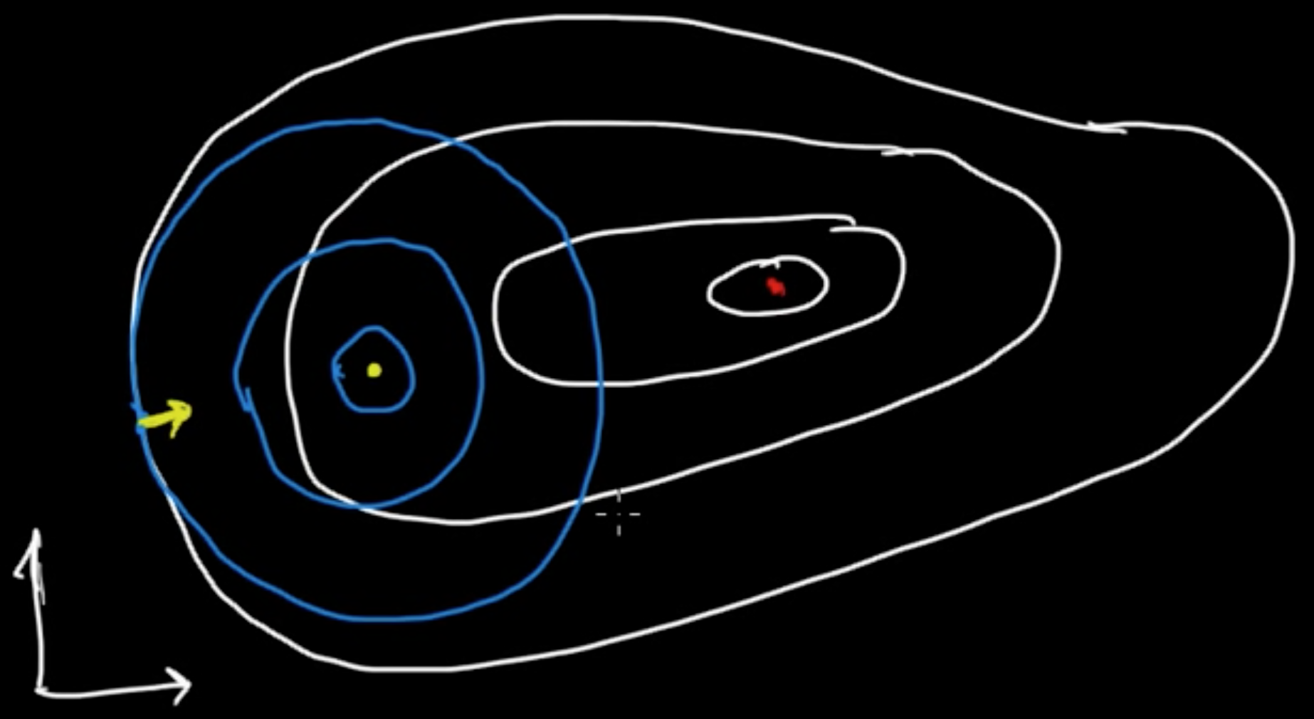
(ML 15.2) Newton’s method (for optimization) in multiple dimensions
Idea: “Make a 2nd order approximation and minimize tha.”
Let $f: \mathbb{R}^n \rightarrow \mathbb{R}$ be (sufficiently) smooth.
Taylor’s theorem: for $x$ near a, letting $g = \nabla f(a)$ and $H = \nabla^2f(a) = \left(\frac{\partial^2}{\partial x_i \partial x_j}f(a)\right)_{ij}$,
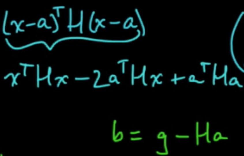
Minimize: $0 = \nabla q = Hx + b \Rightarrow x = -H^{-1}b = a -H^{-1}g$
Critical to check: $\nabla^2 q = H$ $\Rightarrow$ minimum if $H$ is PSD.
Algorithm.
- Initialize $x \in \mathbb{R}^n$
- Iterate: $x_{t+1} = x_t - H^{-1}g$ where $g = \nabla f(x_t), H = \nabla^2 f(x_t)$
Issues.
- $H$ may fail to be PSD. (Option: switch gradient descent. A smart way to do it: Levenberg–Marquardt algorithm)
- Rather than invert $H$, sove $Hy = g$ for $y$, then use $x_{t+1} = x_t - y$. (More robust approach)
- $x_{t+1} = x_t - \alpha_t y$. (small “step size” $\alpha_t>0$)
(ML 17.1) Sampling methods - why sampling, pros and cons
Why sampling?
- For approximate expectations (estimate statistics / posterior infernce i.e. computing probability)
- For visualization
Why expectations?
- Any probability is an expectation: $P[X \in A] = E[I(X \in A)]$.
- Approximation is needed for intractable sums/integrals (can be expressed as expectations)
Pros.
- Easy (both to implement and understand)
- General purpose
Cons.
- Too easy - used inappropriately
- Slow
- Getting “good” samples may be dificult
- Difficult to assess
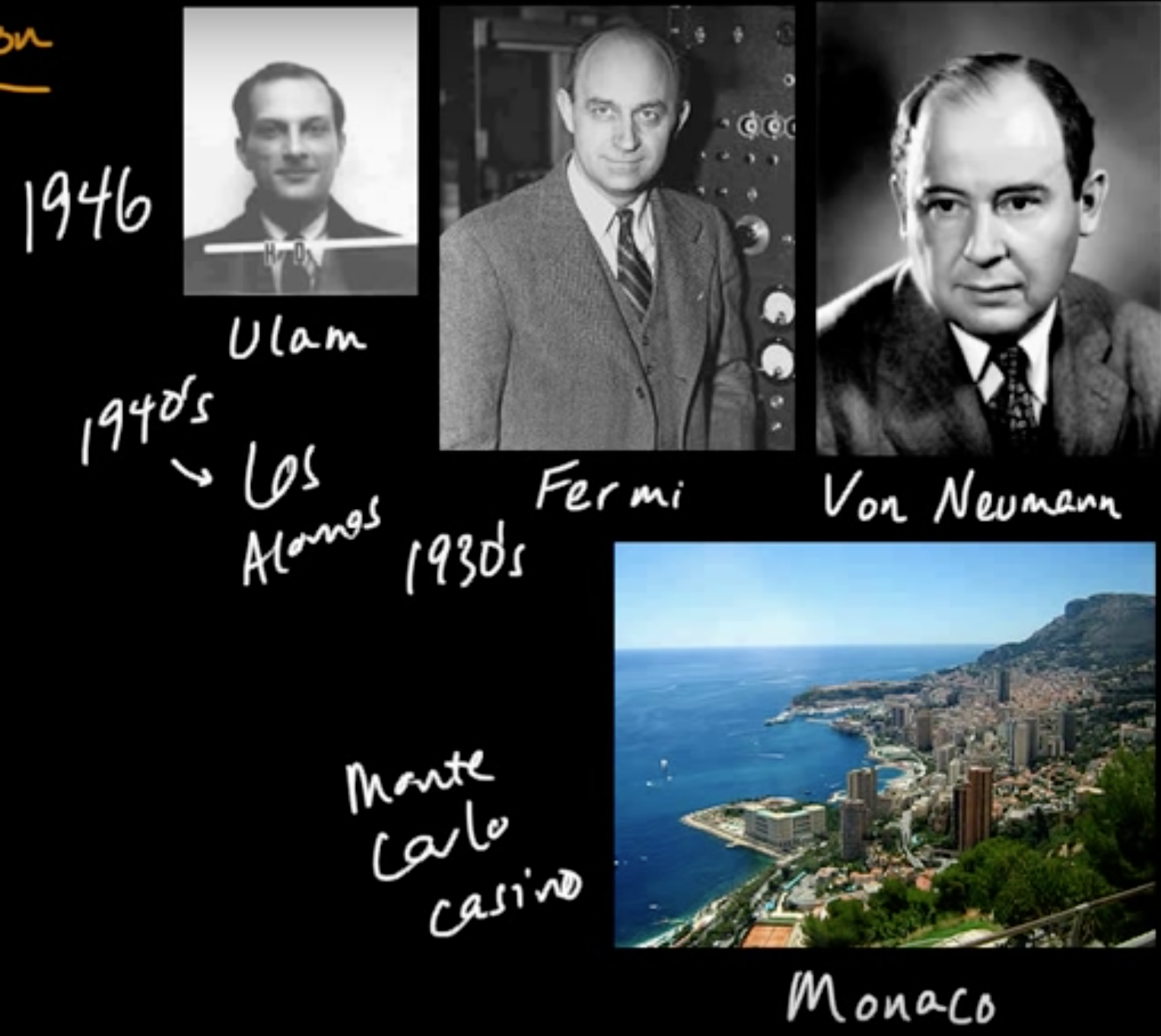
(ML 17.2) Monte Carlo methods - A little history
(ML 17.3) Monte Carlo approximation
Goal: Aprroximate $E[f(X)]$, when intractable.
Definition (Monte Carlo estimator): If $X_1, \ldots, X_n \sim p$ iid then
is a (basic) Monte Carlo estimator of $E[f(X)]$ where $X \sim p$. (sample mean)
Remark
(1) $E[\hat{\mu}_n] = E[f(X)]$ (i.e. $\hat{\mu}_n$ is an unbiased estimator)
(2)
(ML 17.5) Importance sampling - introduction
It’s not a sampling method but an estimation technique!
It can be thought of as a variant of MC estimation.
Recall. MC estimation (by sample mean):
under the BIG assumtion that $X \sim p$ and $X_i \sim p$.
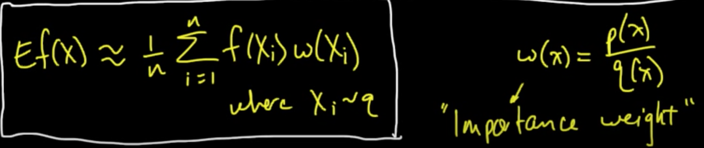
Can we do something similar by drawing samples from an alternative distribution $q$?
Yes, and in some cases you can do much much better!
Density $p$ case.
holds for all pdf $q$ with respect to wchi $q$ is absolutely continuous, i.e., $p(x) = 0$ whenever $q(x)= 0$.
(ML 17.6) Importance sampling - intuition
What makes a good/bad choice of the proposal distrubution $q$?
To be added..
Subscribe via RSS