Notes on Machine Learning 7: Bayesian Inference

(ML 7.1) Bayesian inference - A simple example

“Put distributions on everything, and then use rules of probability!”

Exampl. $D= (x_1, x_2, x_2) = (101, 100.5, 101.5)$ ($n=3$)
$X \sim N(\theta, 1)$ iid given $\theta$

$\theta_{\rm MLE} = \overline{x} = \frac{1}{n}\sum_{i=1}^n = 101$

$ $

$\theta = N(100,1)$ prior
$\theta_{\rm MAP} = 100.75$
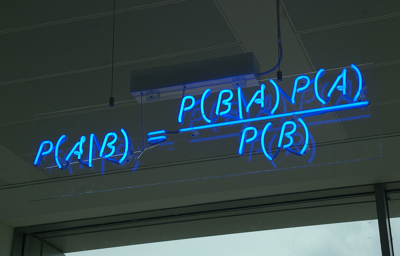
To compute $P(\theta < 100 \vert D)$, one needs posterior $p(\theta \vert D)$

posterior:
$p(\theta \vert D) = \frac{p(D\vert \theta)p(\theta)}{p(D)} = \frac{\prod_{i=1}^np(x_i \vert \theta) p(\theta)}{p(D)}$
$\leadsto$ can be desribed as a normal distribution and so analytically computable!

predictive:
$p(x \vert D) = \int p(x, \theta \vert D) d \theta = \int p(x\vert\theta)p(\theta \vert D) d \theta$
$\leadsto$ analytically integrable!

(ML 7.2) Aspects of Bayesian inference

• Bayesian inference : Assume a prior distribution $p(\theta)$ and then use probability rules to work with $p(x\vert \theta)$ to anser questions.

• Bayesian procedures : Minimize expected loss (averaging over $\theta$).

• Objective Bayesian : use belief-based priors
• Subjective Bayesian : use non-informative priors

Pros.

• Directly answer certain questions, e.g., can compute $P(99 < \theta < 101)$
• Avoid some pathologies (associated with frequentist approach)
• Avoid overfitting
• Automatically do medel selection (“Occam’s razor”)
• Bayesian procedures are often admissible

Cons.

• Must assume a prior
• Exact computation (of posterior) can be intractable ($\leadsto$ have to use approximation)

Priors.

• Non-informative
• Improper, e.g., $p(\theta) = 1$ with density
• Conjugate

(ML 7.3) Proportionality

“Using proportionality is a extraordinarily handy trick (big time-saver) when doing Bayesian inference.”

Notation. $f \propto g$ if there exists $c \neq 0$ such that $g(x) = cf(x)$ for all $x$.

Claim. If $f$ is a PDF and $f \propto g$ then $g$ uniquely determine $f$, and $f(x) = \frac{g(x)}{\int g(x)}dx$.

Proof. $\frac{g(x)}{\int g(x)}dx = \frac{cf(x)}{\int cf(x)}dx = f(x)$.

(ML 7.4) Conjugate priors

Definition. A family $\mathscr{F}$ of (prior) distributions $p(\theta)$ is conjugate to a likelihood $p(D\vert \theta)$ if the posterior $p(\theta \vert D)$ is in $\mathscr{F}$.

Examples.

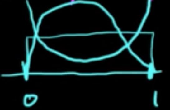
• Beta is conjugate to Bernoulli.
• Gaussian is conjugate to Gaussian (mean).
• Any exponential family has a conjugate prior.

(ML 7.5) (ML 7.6) Beta-Bernoulli model

For example, we model a sequence of binary outcomes, like coin flips, as Bernoulli random variables with Beta prior distribution on the probability of the heads. In other words, Beta is a conjugate prior for Bernoulli.

Setup: $X_1, \ldots, X_n \sim {\rm Bern}(\theta)$ independen gieven $\theta$ with prior $\theta \sim {\rm Beta}(a,b)$.
Here the parameters $a, b$ of the prior are called hyperparameters.

For generaic $X \sim {\rm Bern}(\theta)$, we have

where

From the setup we generate data $D = (x_1, \ldots, x_n)$. Then it’s easy to compute the posterior distribution:

where $n_1 := \sum I(x_i=1)$ and $n_0 := \sum I(x_i=0)$.

Thus, $p(\theta\vert D) = {\rm Beta}(\theta\vert a+n_1, b+n_0)$, and so Beta is conjugate to Bernoulli.

See Beta distribution - an introduction by Ox educ for intuition behind Beta prior.

If $\theta \sim {\rm Beta}(a, b)$, one has:

• $\mathbb{E}(\theta) = \frac{a}{a+b}$;
• $\sigma^2(\theta) = \frac{ab}{(a+b)^2(a+b+1)}$;
• mode $=\frac{a-1}{a+b-2}$.
  ($a+n_1, b+n_0$ are called pseudocounts)

For $\theta \vert D \sim {\rm Beta}(\theta\vert a+n_1, b+n_0)$, on has:

• $\mathbb{E}(\theta\vert D) = \frac{a+n_1}{a+b+n}$;
• mode $=\frac{a+n_1-1}{a+b+n-2}$.

Now let’s make a few connections. We know that

• $\theta_{\rm MLE} =$ empirical probability $= \frac{n_1}{n}$ / $\left(\frac{n_0}{n}, \frac{n_1}{n}\right)$
• $\theta_{\rm MAP} = \frac{a+n_1-1}{a+b+n-2}$

posterior mean $=\frac{a+n_1}{a+b+n} = \frac{a+b}{a+b+n}\cdot \frac{a}{a+b} + \frac{n}{a+b+n}\cdot \frac{n_1}{n}$,
i.e., a convex combination of prior mean & MLE

• When $n \rightarrow \infty$, posterior mean convergees to the MLE.
• When $n = 0$, if we have no data, we get back to the prior mean.

Let’s compute now the (posterior) predictive distribution:

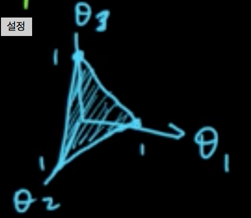
(ML 7.7.A1) Dirichlet distribution

Dirichlet, one of the great mathematicians in 1800s.

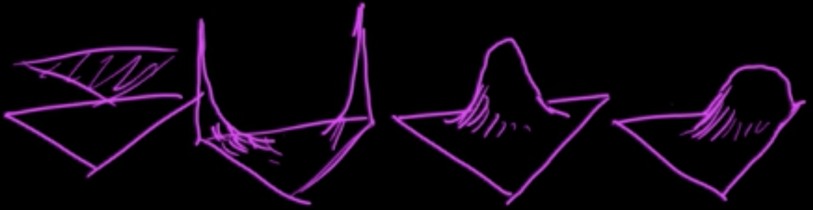
Dirichlet distribution is a distribution on probability distributinos.

$\theta = (\theta_1, \ldots, \theta_n) \sim {\rm Dir}(\alpha)$ means:

where $\alpha = (\alpha_1, \ldots, \alpha_n)$, $\alpha_i >0$ are the parameters, $S = \{x \in \mathbb{R}^n: x_i \ge 0, \sum_{i=1}^n x_n =1 \}$ is the probability simplex, and $\frac{1}{B(\alpha)} =\frac{\Gamma(\alpha_0)}{\Gamma(\alpha_1)\cdots\Gamma(\alpha_n)}$.

$E(\theta_i) = \frac{\alpha_i}{\alpha_0}$

${\rm mode} = \left(\frac{\alpha_1-1}{\alpha_0}, \ldots, \frac{\alpha_n-1}{\alpha_0-n}\right)$

$\sigma^2(\theta) = \frac{\alpha_i(\alpha_0-\alpha_i)}{\alpha_0^2(\alpha_0+1)}$

(7.8)

(ML 7.9) (ML 7.10) Posterior distribution for univariate Gaussian

Given data $D = (x_1, \ldots, x_n)$ with $x_i \in \mathbb{R}$,
want to know from which distribution $D$ might come fomm.
Model $D$ as $X_1, \ldots, X_n \sim N(\mu, \sigma^2)$ for some $\mu, \sigma \in \mathbb{R}$,
i.e., $N(\mu, \sigma^2)$ is the “true” distribution wa want.
Becasue we do not know $\mu$, we model it as a random variable $\theta$, which itself follows a normal distribution:

We assume that $\sigma^2, \mu_0, \sigma_0^2$ are known to make the problem (more) tractable.

Then the postesior distribution is given by

Now,

We have:

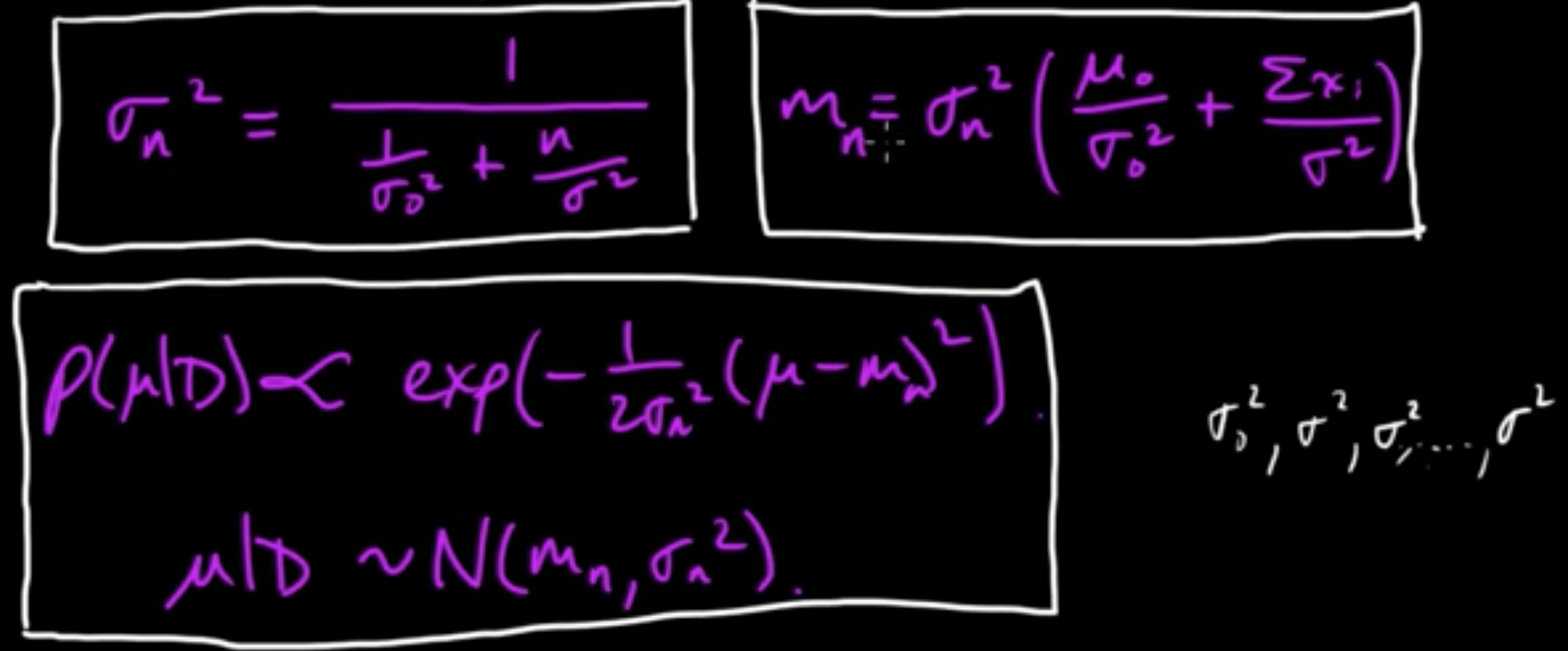
and

with

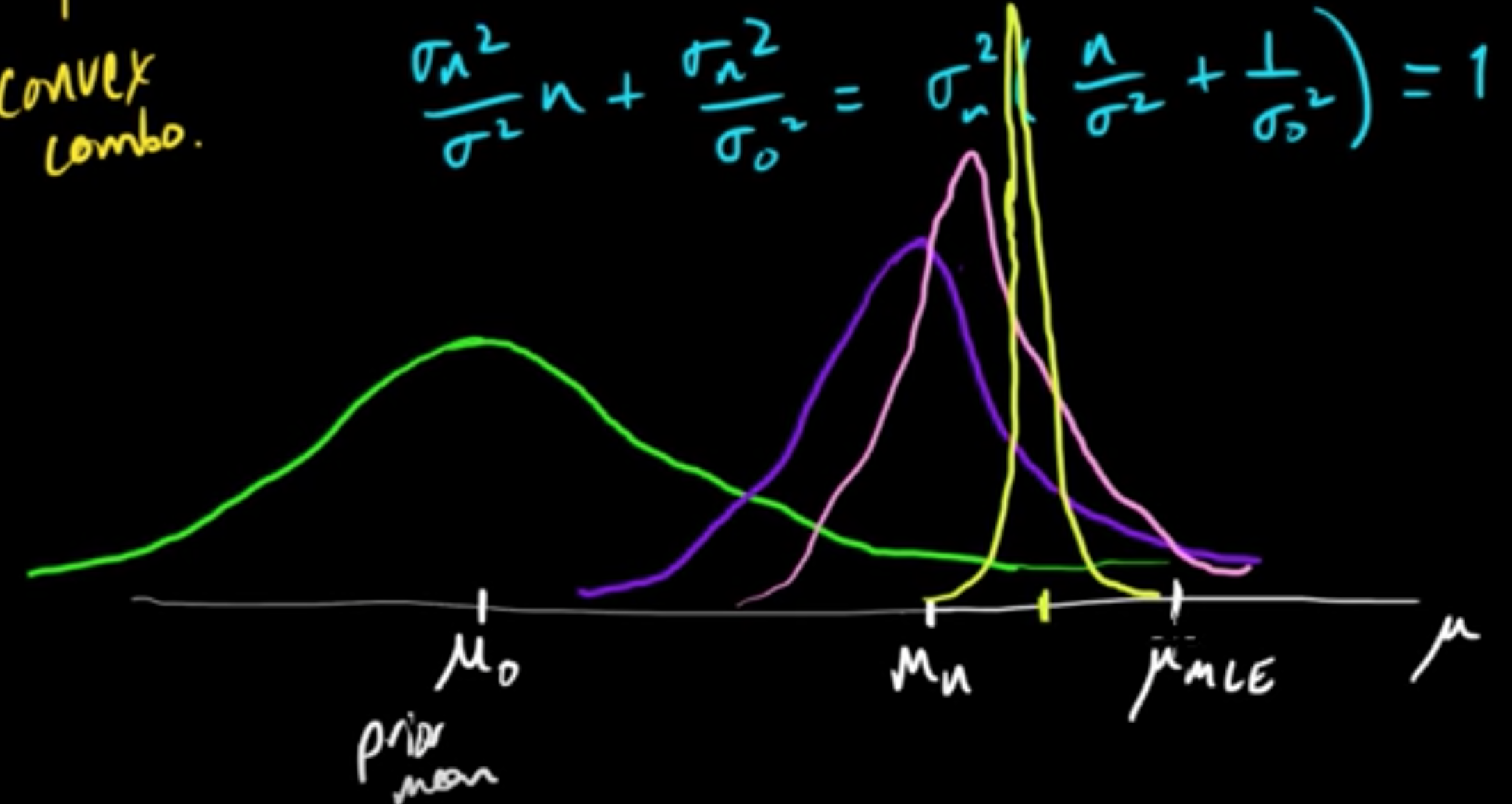
The convergence behavior of the posterior mean (MAP) when $n$ approaches $\infty$: