Notes on Machine Learning 3: Decision theory

(ML 3.1) Decision theory (Basic Framework)

Idea. “Minimize expected loss”

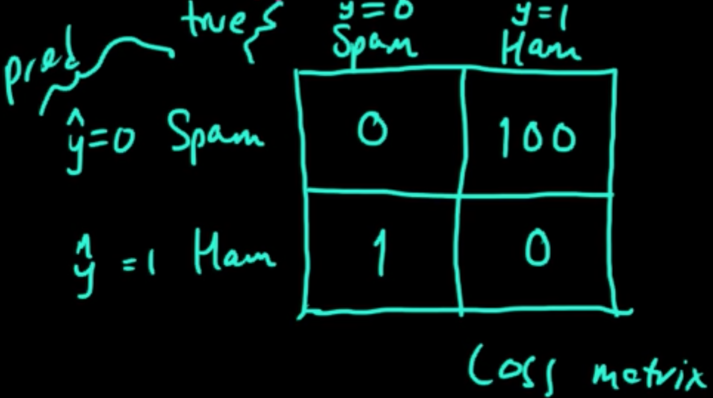
Example. Spam (classification): $x, y, \hat{y}$

Loss function $L(y, \hat{y}) \in \mathbb{R}$

Loss can be thought of as reward or utility depending on the sign of the value.

General framework:

State $s$ (unknown)
Observation (known) e.g, $x$
Actoin $a$
Loss $L(s, a)$

“$0$-$1$ loss”: $L(y, \hat{y}) = I(y\neq \hat{y}) = \begin{cases} 1, \, {\rm if} \,\,\, y=\hat{y}\\ 0, \, {\rm otherwise} \end{cases}$

“Square loss”: $L(y, \hat{y}) = (y-\hat{y})^2$

(ML 3.2) Minimizing conditional expected loss

Decision theory for supervised learning: $D = ((x_1, y_1), \ldots, (x_n, y_n))$, $x, y, \hat{y}$

Given $x$, minimize $L(y, \hat{y}) \ldots$ but we don’t know $y$!
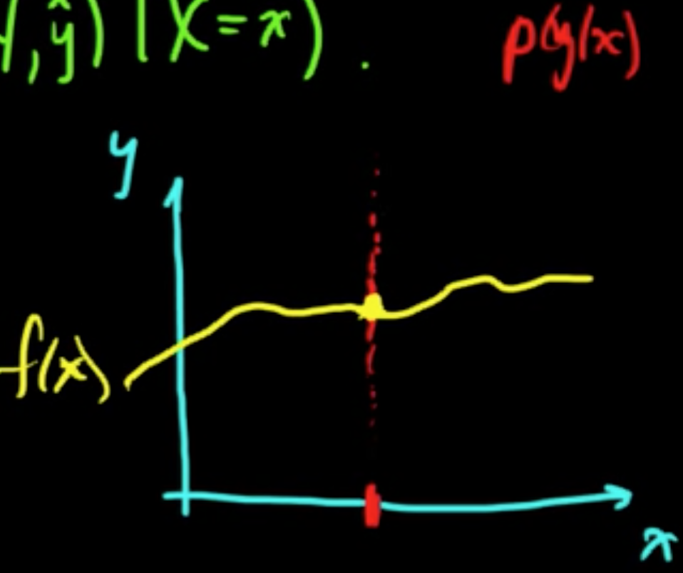
Choose $f$ ($f(x)=y$) to minimize $L(y, f(x)) \ldots$ but don’t knw $x$ or $y$.

Both are ill-posed!

Small loss on average (Probability will come to the rescue!)
Put a probability distribution on theses: $(X, Y) \sim p$
1. Minimizing

$E(L(Y, \hat{y})\vert X= x) = \sum_{y \in Y} L(y, \hat{y})p(y\vert x)$

is now a well-posed problem!

“0-1” loss:
$E(L(Y, \hat{y})\vert X= x)) = \sum_{y \neq \hat{y}} p(y\vert x)) = 1 - p(\hat{y}\vert x)$

$\hat{y} = \arg\min_y E(L(Y, y)\vert X = x)) = \arg\max_y p(y\vert x)$

$p(y\vert x)$ is the key quantity that we need to solve the problem!

(ML 3.3) Choosing $f$ to minimize expected loss

2. $\hat{Y} = f(X)$ (classification, discrete for now)

Want to minimize:

$\begin{aligned} E(L(Y, \hat{Y})) &= E(L((Y, f(X)) = \sum_{x, y}L(y, f(x))p(x, y) \\ &= \sum_x\left(\sum_y L(y, f(x))p(y\vert x)\right)p(x) \\ &= \sum_{x}g(x, f(x))p(x) \\ &= E^Xg(X, f(X)), \end{aligned}$

which is the expecteation for the marginal distribution (by factoring $p(x, y) = p(y\vert x)p(x)$ and letting $g(x) = \sum_y L(y, f(x))p(y\vert x)$).

Suppose for some $x_0, t$ we have $g(x_0, f(x_0)) > g(x_0, t)$.

Define $f_0(x) = \begin{cases} f(x), \, {\rm if} \,\,\, x \neq x_0 \\ t, \, {\rm if} \,\,\, x = x_0. \end{cases}$

Note that $g(x, f(x)) \ge g(x, f_0(x))$ for all $x$.

Then we have

$E(L(Y, \hat{Y})) = E^X(g(X, f(X))) \ge E^X(g(X, f_0(X))) \ge E^X(g(X, f^*(X)))$

Now let’s just go ahead and choose $f^*$ to minimize $g(x, f(x))$:

$f^*(x) = \arg\min_t g(x, t),$

so that $E^X(g(X, f(X))) \ge E^X(g(X, f^*(X)))$ for all $f$.

Again $p(y\vert x)$ is the key quantity.

A nice observation that is called the law of iterated expectation (LIE):

$E(L(Y, \hat{Y})) = E^X(E(L(Y, \hat{Y})\vert X))$

For LIE in general, see: Law of Iterated Expectations.

(ML 3.4) Square loss

$L(y, \hat{y}) = (y-\hat{y})^2$, $(X, Y) \sim p$, $x$ (regression)

Wanna minimize $E(L(Y, \hat{y})\vert X = x) = \int L(Y, \hat{y}) p(y\vert x) dy = \int (y-\hat{y})^2 p(y\vert x) dy$

Assuming enough smoothness of the integrand,

$\begin{aligned} 0 &= \frac{\partial}{\partial y} E(L(Y, \hat{y})\vert X = x) \\ & = \int \frac{\partial}{\partial y} (y-\hat{y})^2 p(y\vert x) dy \\ & = \int 2(y-\hat{y})p(y\vert x) dy \\ & = 2\hat{y} \int p(y\vert x)dy - 2\int y p(y \vert x) dy \\ & = 2\left( \hat{y} - E(Y \vert X = x) \right) \end{aligned}$

gives the only critical point $\hat{y} = E(Y \vert X = x)$ and it tunrs out to give the minimum by looking at the second derivative, which is $2$.

Thus, $E(Y \vert X= x) = \arg\min_y E(L(Y, \hat{y}) \vert X = x)$

With regard to the problem of (ML 3.3):

$f(x) = E(Y \vert X = x)$

(ML 3.5) The Big Picture (part 1)

Goal: Minimize

$E(L(Y, f(X)))$

using the obsrved $p(y\vert x)$ as the key quantities. (Decision-theoretic idea)

EL: Expected Loss
$y$: true value
$f(x)$: our prediction

Core concepts and methods in ML fall out naturally from trying to achieving this goal.

Data: $D = ((x_1, y_), \ldots, (x_n, y_n))$

Discriminative Estimate $p(y\vert x)$ directly using $D$.

$k$NN
Trees
SVM

Generative Estimate $p(y, x)$ using $D$, and then recover $p(y\vert x) = \frac{p(x, y)}{p(x)}$.

Remark While it is much easier to estimate $p(y \vert x)$ than $p(x, y)$ from a statistical perspective, $p(x, y)$ is a richer sort of model.

Parameters / Latent variables $\theta$ introduced, and then consider $p_\theta(x, y) = p(x, y \vert \theta)$

$p(y\vert x, D) = \int p(y\vert x, D, \theta) p(\theta\vert x, D) d\theta$

treating data $D$ as RVs.

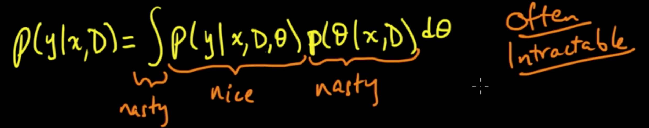
$p(y\vert x, D, \theta)$ : nice in the sense that a closed form expression can be obtained
$p(\theta\vert x, D)$ : often times nasty
$\int /\sum$ : nasty

As a whole computing $p(y \vert x, D)$ is often intractible. Many of the techniques in ML come in the course of different ways to solve (parts of) this problem of computation.

An interesting read I encountered while searching for related resources:
What landmarks are, and why they are important

(ML 3.6) The Big Picture (part 2)

Core ideas & methods of ML: (not necessarily disjoint)

Exact inference (usually not possible)
- Multivariate Gaussian (very nice) / Conjugate priors / Graphical models (use DP)
Point estimates of $\theta$ (simplest)
- MLE / MAP (Maximum A Posteriori)
  [$\theta_{\rm MAP} = \arg\max_\theta p(\theta \vert x, D), p(y \vert x, D) \approx p(y \vert D, \theta_{\rm MAP})$]
- Optimization / EM (Expectation Maximization) / (Empirical Bayes)
Deterministic Approximation
- Laplace Approximation / Variational methods / Expectation Propagation
Stochastic Approximation (very popular, typically very simple to implement)
- MCMC (Gibbs sampling, MH) / Importance Sampling (Particle filter)

(ML 3.7) The Big Picture (part 3)

The problem of Density estimation (Unsupervised)

Data: $D = (X_1, \ldots, X_n), X_i \in \mathbb{R}^d$, iid.

Goal: Estimate the distribution.

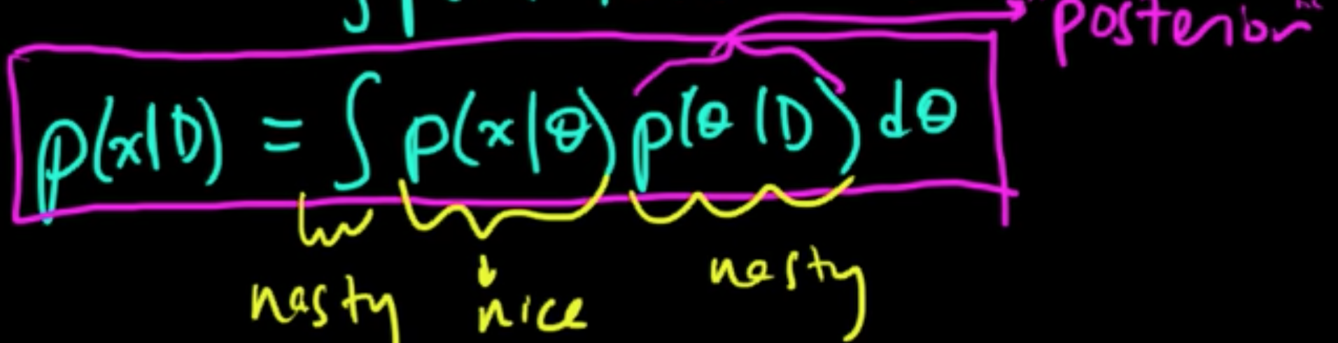
Introduce paramaters $\theta$ as RVs parametrizing $p_\theta$ ($p_\theta(x) = p(x \vert \theta)$)

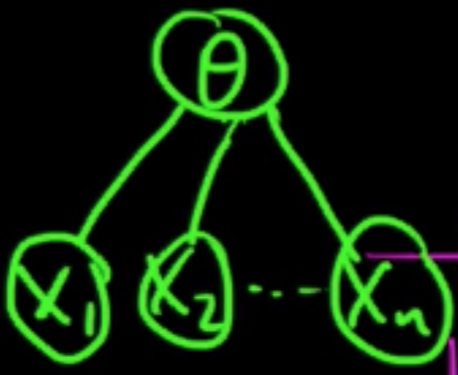
Then $p(x \vert D) = \int p(x, \theta \vert D)d\theta = \int p(x \vert \theta, D) p(\theta \vert D)d\theta = \int p(x \vert \theta) p(\theta \vert D)d\theta$