Notes on Machine Learning 2: Decision trees

(ML 2.1) Classification trees (CART)

CART (Classification And Regression Trees) by Breiman et. al.
(see: https://rafalab.github.io/pages/649/section-11.pdf)

Conceptually very simple approach to classification and regression.
Can be extremely powerful, specially coupled with some randomizaiton technique, and essentially give the best performance.

Main idea: Form a binary tree (by binary splits), and minimize error in each leaf.

Example. (Classification tree)

Data set: $D = ((x_1, y_1), \ldots, (x_n, y_n))$ ($x_i \in \mathbb{R}^2, y \in \{0, 1\}$.

New data point: $x$

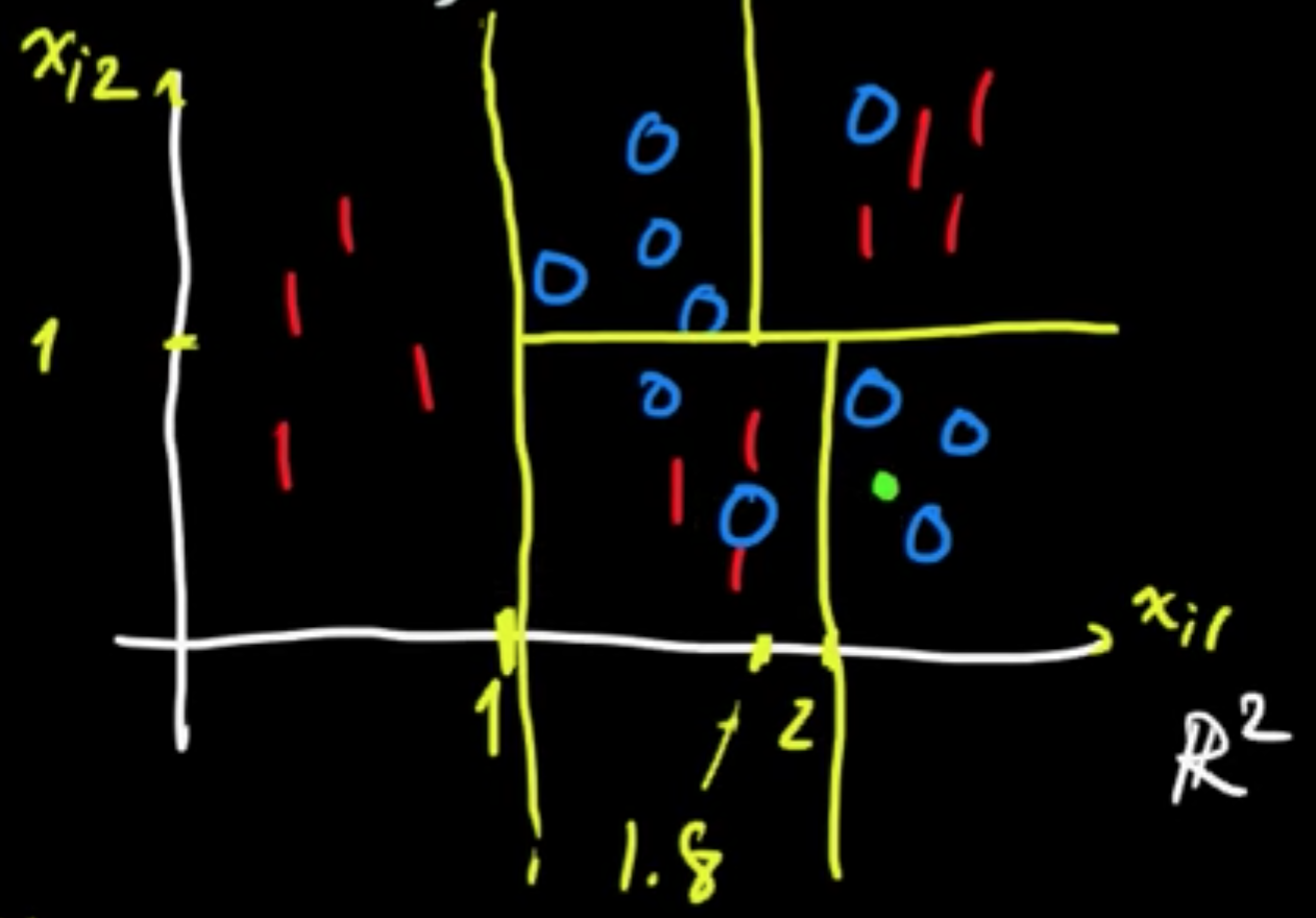
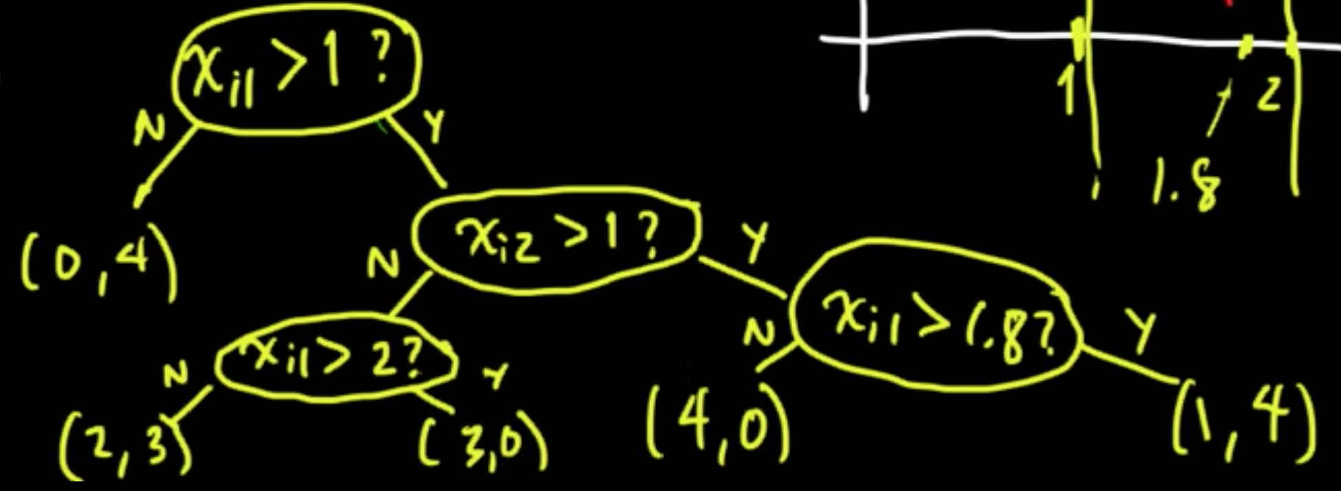
The process defines a function $y = f(x)$ that is constant on each of the petitioned regions.

(ML 2.2) Regression trees (CART)

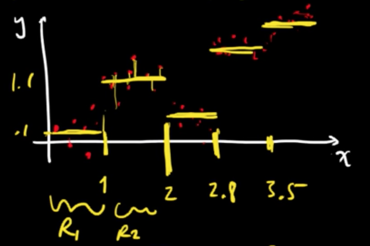
Regression tree ($x_i \in \mathbb{R}, y_i \in \mathbb{R}$)

$\hat{y} = \arg\max_y \sum_{i \in R_1}(y - y_i)^2$

$\Rightarrow \hat{y} =$ average of the $y_i$’s

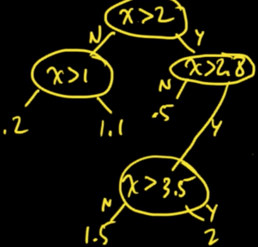
The process defines a function $y = f(x)$ that is piecewise constant.

(ML 2.3) Growing a regression tree (CART)

“Greedy” approach.

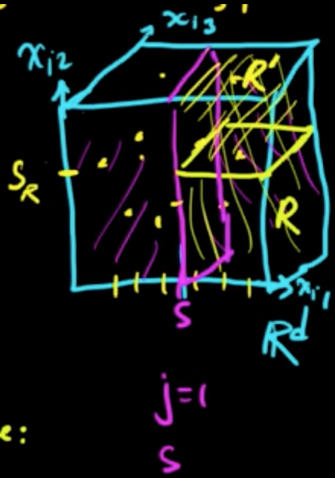
First split. Choose $j$ and $s$ to minimize the following:

Splitting region $R$. Choose $j$ and $s$ to minimize the following:

Stopping criteria::

1. Stop when only one point in $R$.
2. Only consider splits resulting in regions with $\ge m$ (say $m=5$) points per region.

Typically, people use “pruning” strategy.
We’re gonna take “random forest” approach instead.

(ML 2.4) Growing a classification tree (CART)

Datat set: $(x_1, y_1), \ldots, (x_n, y_n)$

$E_R =$ fraction of points $x_i \in R$ misclassified by a majority vote in $R$
$\, \, \, \, \, \, \, \, $ $= \min_y \frac{1}{N}\sum_{i: x_i \in R} I(y_i\neq y)$, $N_R =$ #$\{i : x_i \in R\}$

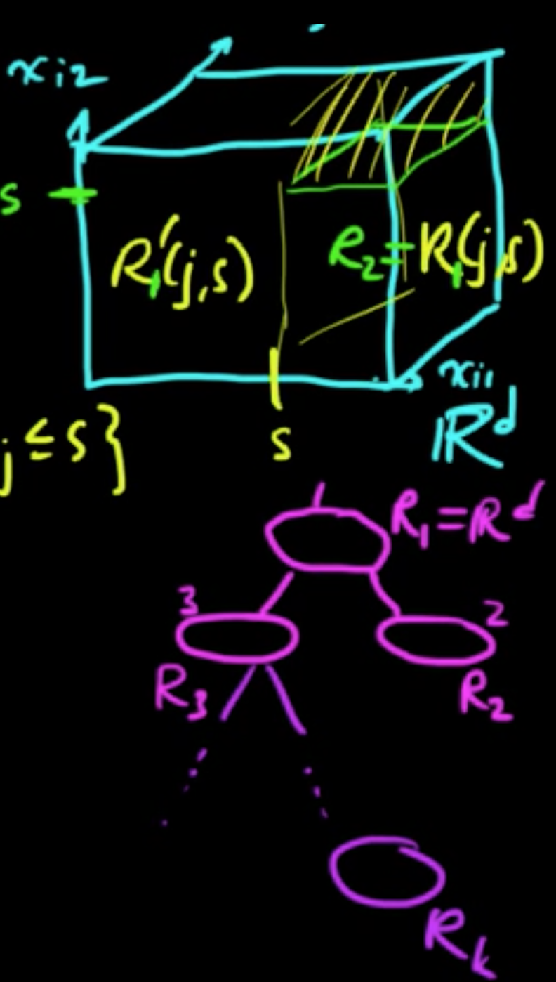
First split. Choose $j$ and $s$ to minimize the following:

where $R_1(j, s) = \{x_i : x_{ij} >s\}, R_1’(j, s) = \{x_i : x_{ij} \le s\}$

Let $R_2 = R_1(j, s), R_3 = R_1’(j,s)$

Splitting $R_k$. Choose $j$ and $s$ to minimize the following:

where $R_k(j, s) = \{x_i \in R_k : x_{ij} >s\}, R_k’(j, s) = \{x_i \in R_k : x_{ij} \le s\}$

Stopping criteria:

1. Stop when only one point in $R$.
2. Only consider splits resulting in regions with $\ge m$ (say $m=5$) points per region.
3. Stop when $R_k$ contains only points of one class.

Use when minimizing?

1. Entropy
2. Gini index

(ML 2.5) Generalizations for trees (CART)

Imputiry measures for classification:

1. Misclassification rate $E_R$
2. Entropy

where $\mathscr{Y}$ is a finite set of (possible) classes and $p_R$ empirical distribution.

The idea of entropy : want to choose splits in which each of the regions are as homogenous as possible.

1. “Gini index”

Remark

1. $H_R$ and $G_R$ tend to work better than $E_R$.
2. $G_R$ has some nice analytical properties that makes it easier to work with.

HTR (The Elements of Statistical Learning by Trevor Hastie, Robert Tibshirani, Jerome Friedman)

• Categorical predictors
• Loss matrix
• Missing values
• Linear combinations
• Instability

(ML 2.6) Bootstrap aggregation (Bagging)

A fantastic technique for taking a classifier and making it better (By Breiman)

Bagging for Regression.

$D = \{ (X_1^{(1)}, Y_1^{(1)}), \ldots, (X_n^{(1)}, Y_n^{(1)}) \}$ $\sim P$ iid

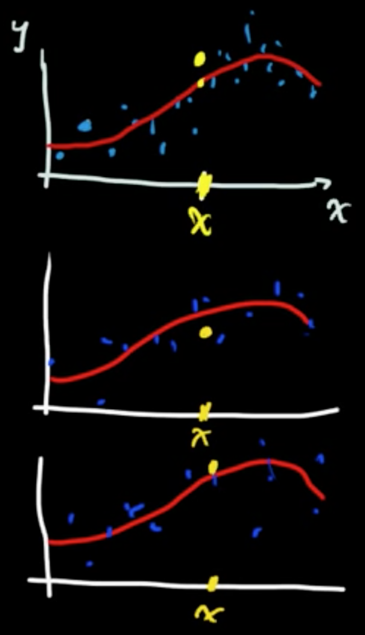
Given a new point $x$, predict $Y^{(1)}$ ($f(x) = y$)

From the given sample, uniformly sample with replacement to obtain:

$(X_1^{(2)}, Y_1^{(2)}), \ldots, (X_n^{(2)}, Y_n^{(2)})$ $Y^{(2)}$

$\cdots$

$(X_1^{(m)}, Y_1^{(m)}), \ldots, (X_n^{(m)}, Y_n^{(m)})$ $Y^{(m)}$

Suppose each esimiator $Y^{(i)}$ has teh correct mean, i.e.,

$EY^{(i)} = y = f(x)$ for each $i \{1, \ldots, m\}$

In other words, they are “unbiased estimators.”

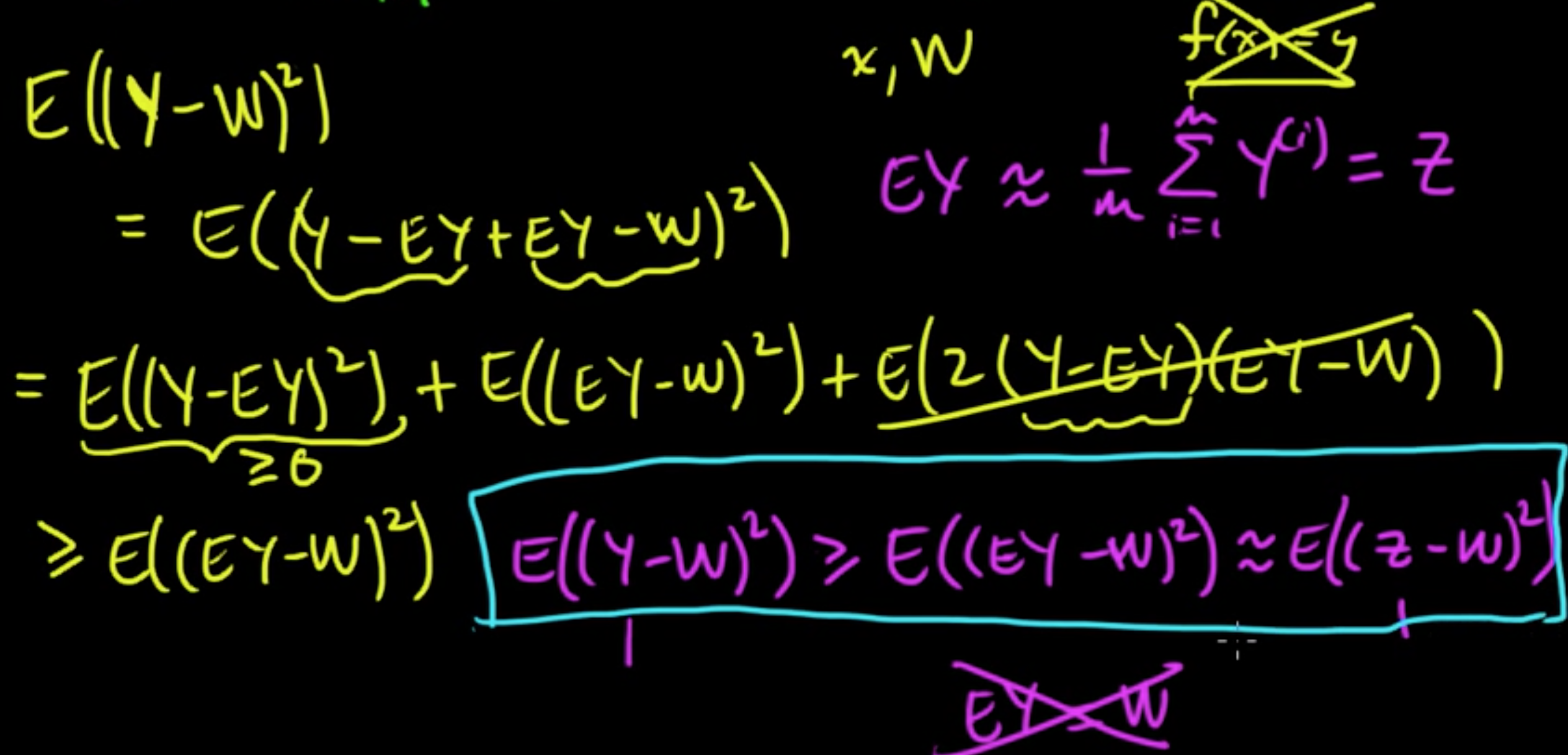
Now we measure our error according to the squared distance from the true value $(Y-y)^2$, which is called a loss function.

Then the risk (i.e. expected loss) is given by

If we define a new RV (this is where the aggregation comes in!)

we get $EZ = \frac{1}{m}\sum y = y$. ($Z$ is also an unbiased estimator!)

Then

Because we just have one data set, we approximae $P$ by the empirical distribution $\hat{P}$ to draw bootstrap samples

$(X_i^{(k)}, Y_i^{(k)}) \sim$ Uniform$(D)$ iid.

(ML 2.7) Bagging for classification

Two essential approaches:

1. Majority vote. For each data set construct a classifier to get a sequence of classifiers $C_1, \ldots, C_n$. Then given a new point $x$, look at the class that each $C_i$ predicted for $x$ and take majority vote.
2. Average estimated probabilities. Th classifiers define $p_x^{(1)}, \ldots, p_x^{(n)}$, (estimated) PMFs on $\mathscr{Y}$. We define

(similar to the regerssion case)

We classify $x$ as the most likely class according to this estimated probability.

Genralization Now let’s see what we can do by dropping the two assumptions $f(x)=y$ and “unbiasedness of classifiers” and only keeping the iid assumption.

Assume we have a new point $x$ and a RV $W$ (true value).

(ML 2.8) Random forests

Also by Breiman

An extremely simple technique with state of the art perfomance

A study by Caruana & Niculescu-Mizil (2006), An Empirical Comparison of Supervised Learning Algorithms, shows:

1. Boosted decition free (another aggregation tree)
2. Random forests
3. Bagged decision tree
4. SVM
5. Neural Nets $\cdots$

$D = ((x_1, y_1), \ldots, (x_n, y_n)$, $x_ \in \mathbb{R}$ (parameters: $B$ and $m<d$)

For $i$ in [1, 2, .. , B]:
$\,\,\,\,\,\,\,\,\,$ Choose bootstrap sample $D_i$ from $D$
$\,\,\,\,\,\,\,\,\,$ Construct tree $T_i$ using $D$ s.t.
$\,\,\,\,\,\,\,\,\,\,\,\,\,\,\,\,\,\,$ At each note, choose random subset (called random subspace) of $m$ features, and only consider splitting on thoese features

Given $x$, take majority vote (for classification) or average (for regression).

Works essentialy for the same reasonas bagging, except that this time averaging over features (called ensemble) reduces the variance of the overall final estimator.