
Notes on Probability Primer 1: Measure theory
by 장승환
(PP 1.1) Measure theory: Why measure theory - The Banach-Tarski Paradox
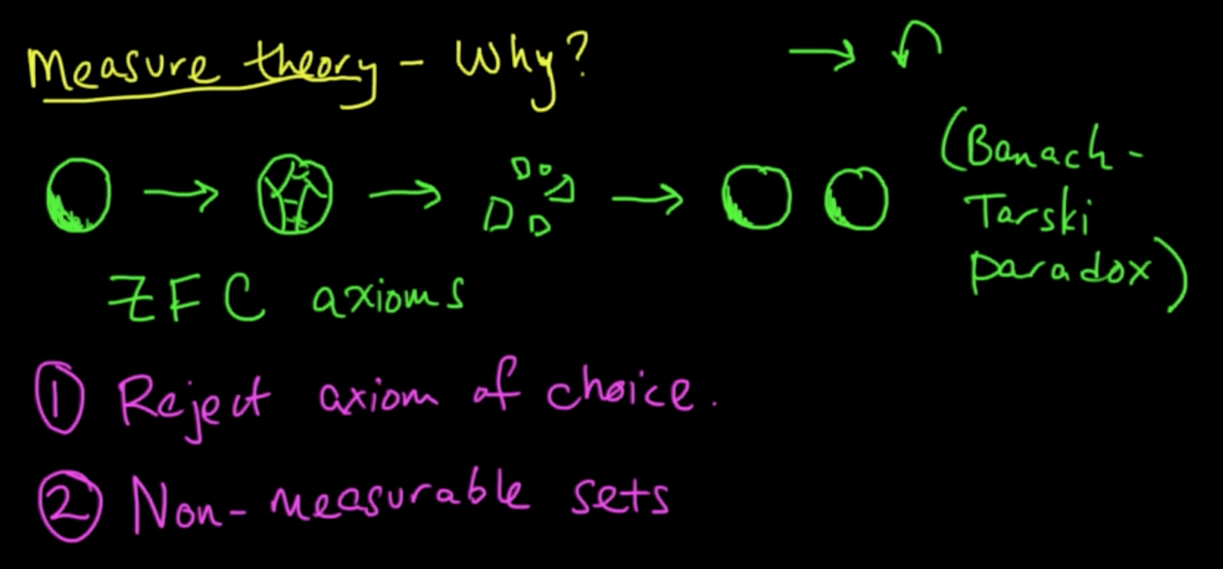
A bit more detailed explanations on the Banach-Tarski paradox here: The Banach–Tarski Paradox.
(PP 1.2) Measure theory: $\sigma$-algebras
Definition. Given a set $\Omega$, a $\sigma$-algebra on $\Omega$ is a nonempty collection $\mathcal{A} \subset 2^{\Omega}$ s.t.
- closed under complements ($E \in \mathcal{A} \Rightarrow E^c \in \mathcal{A}$)
- closed under countable unions ($E_1, E_2, \ldots \in \mathcal{A} \Rightarrow \cup_{i = 1}^\infty E_i \in \mathcal{A}$)
Remark
- $\Omega \in \mathcal{A}$ (some $E \in \mathcal{A}$. $E^c \in \mathcal{A}$. $\Omega = E \cup E^c \in \mathcal{A}$.)
- $\emptyset \in \mathcal{A}$ ($\emptyset = \Omega^c \in \mathcal{A}$)
- $\mathcal{A}$ is closed under countable intersections:
If $E_1, E_2, \ldots \in \mathcal{A}$, then (by De Morgan’s laws)
(PP 1.3) Measure theory: Measures
Definition. Given $\mathscr{C}$ $\subset$ $2^\Omega$, the $\sigma$-algebra generated by $\mathscr{C}$, witten $\sigma(\mathscr{C})$ is the “smallest” $\sigma$-algebra containing $\mathscr{C}$. (That is, $\sigma(\mathscr{C}) = \cap_{\mathcal{A} \supset \mathscr{C}} \mathcal{A}$)
Remark. $\sigma(\mathscr{C})$ always exists because:
- $2^\Omega$ is a $\sigma$-algebra
- any intersection of $\sigma$-algebras is a $\sigma$-algebra
Examples.
- $\mathcal{A} = \{\emptyset, \Omega\}$
- $\mathcal{A} = \{\emptyset, E, E^c, \Omega\}$
- If $\Omega = \mathbb{R}$ then the Borel $\sigma$-algebra is $\mathcal{B} = \sigma(\mathscr{T})$ where $\mathscr{T} =$ $\{$open sets of $\mathbb{R} \}$
Definition. A measure $\mu$ on $\Omega$ with $\sigma$-algebra $\mathcal{A}$ is a function $\mu : \mathcal{A} \rightarrow [0, \infty]$ s.t.
- $\mu(\emptyset) = 0$
- $\mu(\cup_{i=1}^\infty E_i) = \sum_{i=1}^\infty \mu(E_i)$ for any sequence $E_1, E_2, \ldots \in \mathcal{A}$ of pairwise disjoint sets (countable additivity)
Definition. A probability measure is a measure $P$ s.t. $P(\Omega)= 1$
(PP 1.4) Measure theory: Examples of Measures
The defining conditions of a probability measure is called the Kolmogorov’s axioms. (father of modern probability theory)
Examples.
- (Finite set) $\Omega = \{1, \ldots, n\}, \mathcal{A} = 2^\Omega$, $P({k}) = P(k) = \frac{1}{n}$ (gives uniform distribution)
$P(\{1, 2, 4\}) = P(\{1\} \cup \{2\} \cup \{4\})) = P(1) + P(2) + P(4)$ - (Countably infinite) $\Omega = \{1, 2, 3, \ldots \}, \mathcal{A} = 2^\Omega$
$P(k) =$ probability it takes $k$ coinflips to get heads $=\alpha(1-\alpha)^{k-1} = \frac{1}{2}(1-\frac{1}{2})^{k-1}$
(gives gemetric distribution) - (Uncountable) $\Omega = [0, \infty)$, $\mathcal{A} = \mathcal{B}([0, \infty )])$
$P([0, x)) = 1-e^{-x}$ $\forall x>0$ (gives exponential distribution)
Note: $P(\{x\})$ $\forall x>0$ (a symptom of continuous distributions)
(PP 1.5) Measure theory: Basic Properties of Measures
(4) Lebesgue measure (on $\mathbb{R}$). $\Omega, \mathcal{A} = \mathcal{B}(\mathbb{R})$
for any $a, b \in \mathbb{R}, a< b$.
Theorem (Basic properties of measures). Let $(\Omega, \mathcal{A}, \mu)$ be a measure space.
- Monoronicity: If $E, F \in \mathcal{A}$ and $E \subset F$, then $\mu(E) \le \mu(F)$.
- Subadditivity (handy!): If $E_1, E_2, \cdots \in \mathcal{A}$, then $\mu(\cup_{i=1}^\infty E_i) \le \sum_{i=1}^\infty E_i$
(PP 1.6) Measure theory: Basic Properties of Measures (continued)
- Continuity from below: If $E_1, E_2, \cdots \in \mathcal{A}$ and $E_1 \subset E_2 \subset \cdots$, then $\mu(\cup_{i=1}^\infty E_i) = \lim_{i \rightarrow \infty} \mu(E_i)$
- Continuity from above: If $E_1, E_2, \cdots \in \mathcal{A}$ and $E_1 \supset E_2 \supset \cdots$ and $\mu(E_1) < \infty$, then $\mu(\cap_{i=1}^\infty E_i) = \lim_{i \rightarrow \infty} \mu(E_i)$
Properties 3 and 4 are very innocent looking but are essential in proving pretty nontrivial theorems!
(PP 1.7) Measure theory: More Properties of Probability Measures
Facts. Let $(\Omega, \mathcal{A}, P)$ be a probabilistic measure space with $E, F, E_i \in \mathcal{A}$.
- $P(E \cup F) = P(E) + P(F)$ if $E \cap F = \emptyset$
- $P(E \cup F) = P(E) + P(F) - P(E \cap F)$
- $P(E) = 1 - P(E)$
- $P(E \cap F^c) = P(E) - P(E \cap F)$
- (Inclusion-Exclusion formula) $P(\cup_{i=1}^n E_i) = \sum_{i} P(E_i) - \sum_{i<j}P(E_i \cap E_j) + \sum_{i<j<k}P(E_i \cap E_j \cap E_k) - \cdots +(-1)P(E_1 \cap E_2 \cap \cdots E_n)$
- $P(\cup_{i=1}^n E_i) \le \sum_{i=1}^n P(E_i)$ and $P(\cup_{i=1}^\infty E_i) \le \sum_{i=1}^\infty P(E_i)$
(PP 1.8) Measure theory: CDFs and Borel Probability Measures
$\mathbb{R}, \mathcal{B}(\mathbb{R})$, $(a, b)$
Definition. A Borel measure on $\mathbb{R}$ is a measure on $(\mathbb{R}, \mathcal{B}(\mathbb{R}))$
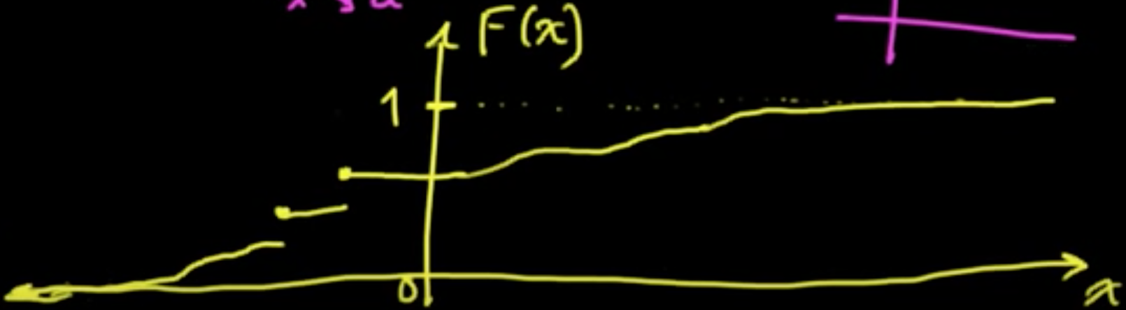
Definition. A CDF (cumulative distribution function) is a function $F : \mathbb{R} \rightarrow \mathbb{R}$ s.t.
- $F$ is nondecreasing ($x \le y \Rightarrow F(x) \le F(y)$)
- $F$ is right continuous ($\lim_{x \rightarrow a^+} = F(a)$)
- $\lim_{x \rightarrow \infty} F(x) = 1$
- $\lim_{x \rightarrow -\infty} F(x) = 0$
Theorem.
- If $F$ is a CDF, then there is a unique Borel probability measure on $\mathbb{R}$ s.t. $P((-\infty, x]) = F(x)$ $\forall x \in \mathbb{R}$
- If $P$ is a Borel probability measure on $\mathbb{R}$, then there is a unique CDF $F$ s.t. $F(x) = P((-\infty, x])$ $\forall x \in \mathbb{R}$
That is, there is an equivalence between CDFs and Borel probability measures.
In sum, CDFs “parametrize” Borel probability measures!
(PP 1.R) References for Probability and Measure theory
Comment.
- Excellent text – right level
- Do the exercises
Reak Analysis. (Undergrad.)
- Rudin’s Principles of Mathematical Analysis
Probability.
- Jacod & Protter Probability Essentials (some of the proofs not very satisfying)
- Durrett Probability Theory & Examples (a bit advanced side)
- Grimmett & Stirzaker Probabilty & Random Processes
Reak Analysis. (Grad.)
- Folland’s Real Analysis
Subscribe via RSS