Notes on Machine Learning 6: Maximum a posteriori (MAP) estimation

(ML 6.1) Maximum a posteriori (MAP) estimation

Setup.

• Given data $D = (x_1, \ldots, x_n)$, $x_i \in \mathbb{R}^d$.
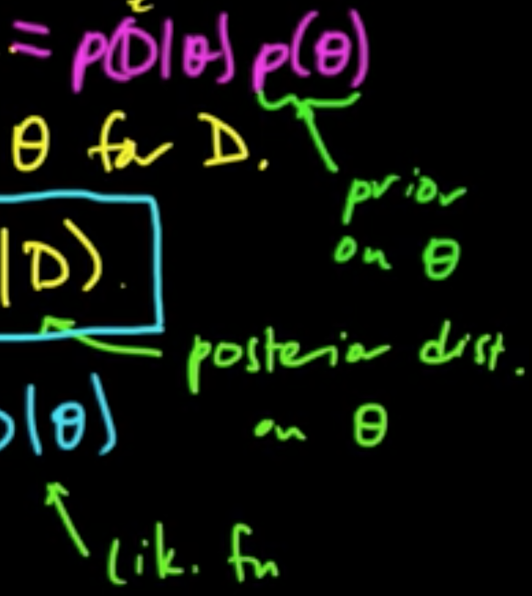
• Assume a jont distribution $p(D, \theta) = p(D\vert \theta)p(\theta)$ where $\theta$ is a RV.
• Goal: choose a good value of $\theta$ for $D$.
• Choose $\theta_{\rm MAP} = \arg\max_\theta p(\theta\vert D)$. $\,$ cf. $\theta_{\rm MLE} = \arg\max_\theta p(D\vert \theta)$.

Pros.

• Easy to compute & interpretable
• Avoid overfitting, closely connected with “regularization”/”shrinkage”
• Tends to look like MLE asymptotically ($n \rightarrow \infty$)

Cons.

• Point estimate - no representation of uncertainty in $\theta$
• Not invariant under reparametrization (cf. $T = g(\theta) \Rightarrow T_{\rm MLE} = g(T_{\rm MLE})$)
• Must assume prior on $\theta$

(ML 6.2) MAP for univariate Gaussian mean

Given data $D = (x_1, \ldots, x_n)$ with $x_i \in \mathbb{R}$.
Suppose $\theta$ is a RV $\sim N(\mu, 1)$ (prior!) and
RVs $X_1, \ldots, X_n \sim N(\theta, \sigma^2)$ are conditionally independent given $\theta$. So we have $p(x_1, \ldots, x_n \vert \theta) = \prod_{i=1}^n p(x_i\vert \theta)$.

Then

To find extreme point, we set

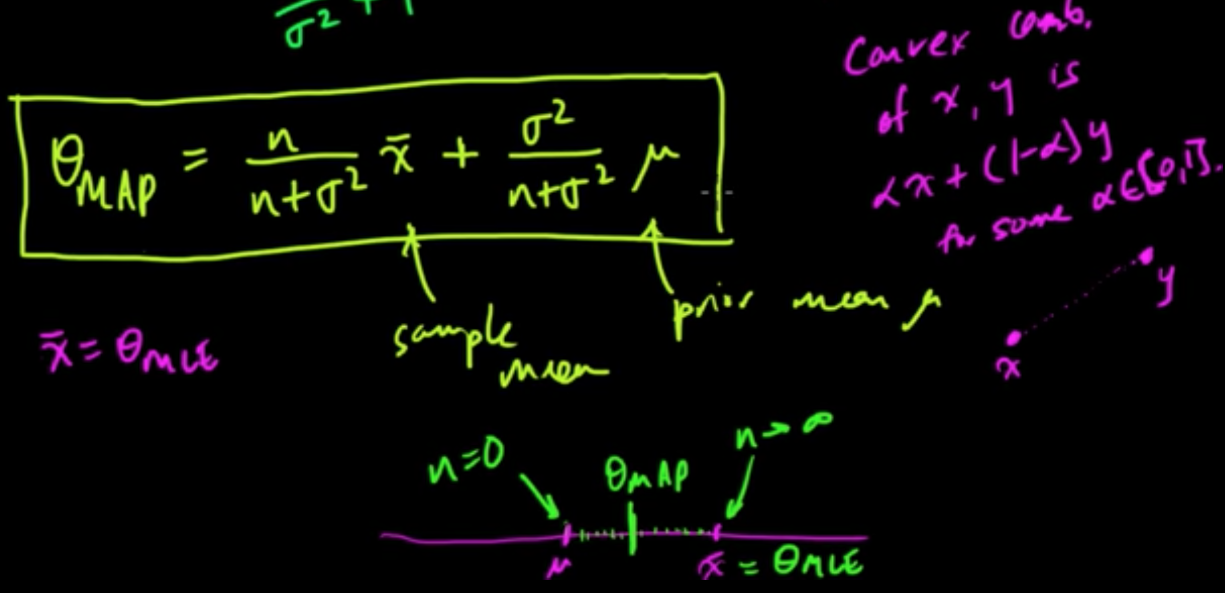
to obtain $\theta = \frac{\sum \frac{x_i}{\sigma^2} +\mu}{\frac{n}{\sigma^2} + 1} = \frac{\sum x_i -\sigma^2\mu}{n + \sigma^2}$.

Then $\,$ $\theta_{\rm MAP} = \frac{n}{n+\sigma^2}\bar{x} + \frac{\sigma^2}{n+\sigma^2}\mu$.

(ML 6.3) Interpretation of MAP as convex combination